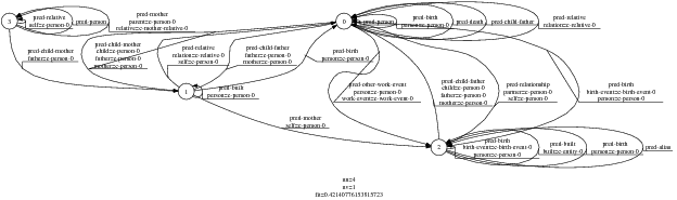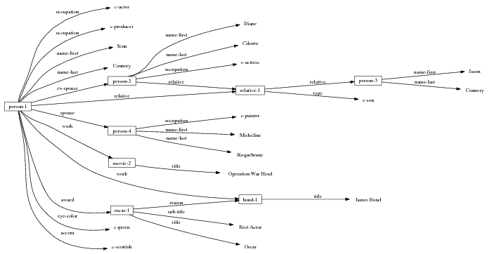
Figure 1.2: Graph Rendering of my Knowledge Representation.
Indirect Supervised Learning of
Strategic Generation Logic
Pablo Ariel Duboue
Submitted in partial fulfillment of the
requirements for the degree
of Doctor of Philosophy
in the Graduate School of Arts and Sciences
COLUMBIA UNIVERSITY
2005
©2005
Pablo Ariel Duboue
All Rights Reserved
Abstract
Indirect Supervised Learning of
Strategic Generation Logic
Pablo Ariel Duboue
The Strategic Component in a Natural Language Generation (NLG) system is responsible for determining content and structure of the generated output. It takes a knowledge base and communicative goals as input and provides a document plan as output. The Strategic Generation process is normally divided into two subtasks: Content Selection and Document Structuring. An implementation for the Strategic Component uses Content Selection rules to select the relevant knowledge and Document Structuring schemata to guide the construction of the document plan. This implementation is better suited for descriptive texts with a strong topical structure and little intentional content. In such domains, special communicative knowledge is required to structure the text, a type of knowledge referred as Domain Communicative Knowledge. Therefore, the task of building such rules and schemata is normally recognized as tightly coupled with the semantics and idiosyncrasies of each particular domain. In this thesis, I investigate the automatic acquisition of Content Selection rules and the automatic construction of Document Structuring schemata from an aligned Text-Knowledge corpus. These corpora are a collection of human-produced texts together with the knowledge data a generation system is expected to use to construct texts that fulfill the same communicative goals as the human texts. They are increasingly popular in learning for NLG because they are readily available and do not require expensive hand labelling. To facilitate learning I further focus on domains where texts are also abundant in anchors (pieces of information directly copied from the input knowledge base). In two such domains, medical reports and biographical descriptions, I have found aligned Text-Knowledge corpus for my learning task. While aligned Text-Knowledge corpora are relatively easy to find, they only provide indirect information about the selected or omitted status of each piece of knowledge and their relative placement. My methods, therefore, involve Indirect Supervised Learning (ISL), as my solution to this problem, a solution common to other learning from Text-Knowledge corpora problems in NLG. ISL has two steps; in the first step, the Text-Knowledge corpus is transformed into a dataset for supervised learning, in the form of matched texts. In the second step, supervised learning machinery acquires the CS rules and schemata from this dataset. My main contribution is to define empirical metrics over rulesets or schemata based on the training material. These metrics enable learning Strategic Generation logic from positive examples only (where each example contains indirect evidence for the task).
This thesis has been possible with the continuous support of many, many friends and colleagues. Sometimes just a word of encouragement, a smile in the corridor was all what it takes to keep the flow of effort through the days.
First and foremost, I would like to thank my family, in special my parents Ariel and Patricia, and my sister Carolina for their continuous support all through the years. I dedicate this thesis to them. To my extended family, in particular to Jaime, Mema, Victor, Ana, Vicky, Conri, Marina, Gusti, also my deepest thanks.
This thesis has been possible through the continuous guidance and support of my advisor, Prof. Dr. Kathleen R. McKeown. I have been blessed of having Kathy as my advisor. She is not only extremely knowledgeable in the subject matter of this dissertation, but I do believe she as also able to let out the best in each of her students. When Kathy speaks, she is the voice of the community speaking. Every time I had to change something in a paper following her advice, I find out later at conferences that her advice was well motivated. For all these years, thanks Kathy.
My thesis committee contained an unusual rainbow of skills that evaluated and contributed criticism to this thesis from different, varied perspectives. The committee chair, Prof. Dr. Julia Hirschberg has asked me some of the toughest research questions I have been asked in my life. Questions that kept me thinking for months. Questions for which I may spend years after having finished this thesis still looking for answers. I am most thankful to Julia for sharing her continuous scientific curiosity with me. My external committee members Prof. Dr. Dan Jurafsky and Dr. Owen Rambow both offered different perspectives over the subjects dealt in this dissertation. Dan made a many comments about the indirect supervised part. His comments helped me shape the problem in the way it is presented today. Owen was the other NLG person in the committee (aside from Kathy). I have admired Owen’s work since my candidacy exam and it has been a pleasure to have him in my committee. Finally, Prof. Dr. Tony Jebara contributed his deep knowledge in Machine Learning in several, different ways. I have learned a lot from Tony, both in the technical aspects of Machine Learning and in the inter-personal issues related to communicating with researchers in that community. I just wish I have had started interacting with Tony earlier in this dissertation. The machine learning part would be definitely better.
Special thanks go for Smara, Michel and Tita. This thesis wouldn’t be here without their continuous support through the years. Seriously. You know that very well. Thanks, thanks, thanks.
To my friends at the CU NLP Group: Michel Galley, Smaranda Muresan, Min-Yen Kan, Noemie Elhadad, Sasha Blair-Goldensohn, Gabriel Illouz, Simone Teufel, Hong Yu, Nizar Habash, Elena Filatova, Ani Nenkova, Carl Sable, Dave Evans, Barry Schiffman, James Shaw, Shimei Pan, Hongyan Jing, Regina Barzilay, Judith Klavans, Owen Rambow, Vassielios Hatzivassiloglou, David Elson, Brian Whitman, Dragomir Radev, Melissa Holcombe, Greg Whalen, Rebecca Passonneau, Sameer Maskey, Aaron Harnly, John Chen, Peter Davis, Melania Degeratu, Jackson Liscombe and Eric Siegel. To the GENIES Team, in special to Andrey Rzhetsky. To the MAGIC Team, in special to Dr. Desmond Jordan. To the Columbia and Colorado AQUAINT team for creating the environment where half of this thesis flourished, in particular to James Martin, Wayne Ward and Sameer Pradham.
To my friends at the Computer Science Department: Amélie Marian (et Cyril!), Sinem Guven, Guarav Kc, Panos (Panagiotis Ipeirotis), Liz Chen, Kathy Dunn, Alpa Shah, Gautam Nair, Anurag Singla, Tian Tian Zhou, Blaine Bell, Rahul Swaminathan, Vanessa Frias, Maria Papadopouli, Phil Gross, Katherine Heller, Jennifer Estaris, Eugene Agichtein and Gabor Blasko thanks for their friendship and support. My deepest thanks to Martha Ruth Zadok, Anamika Singh, Twinkle Edwards, Remiko Moss and Patricia Hervey. To my officemates: Liu Yan, Lijun Tang, dajia xiexie. Special thanks to the professors Luis Gravano, David Sturman, Bernie Yee, Bill Noble, and Sal Stolfo. Finally, to to my former students Howard Chu, Yolanda Washington, Min San Tan Co, Ido Rosen and Mahshid Ehsani, from which I learned much than what they might learned from me, most certainly.
To the many friends at Columbia University that keep me away from screens and keyboards and let me regain some of my lost sanity. Special thanks to Fabi (Fabiola Brusciotti), Sato (Satoko Shimazaki), Cari (Carimer Ortiz), Al (Alberto Lopez-Toledo), Steve (Steven Ngalo), Sila Konur, Daniel Villela, Ana Belén Benítez Jiménez, Gerardo Hernández Del Valle, Victoria Dobrinova Tzotzkova, Raúl Rodríguez Esteban. Also to: Tarun Kapoor, Hui Cao, Tammy Hsiang, Maria Rusanda Muresan, Priya Sangameswaran, Shamim Ara Mollah, Ivan Iossifov, Su-Jean Hwang, Enhua Zhang, Kwan Tong, Barnali Choudhury, Manuel Jesus Reyes Gomez, Isabelle Sionniere.
To the CRF staff, specially Daisy, Mark and Dennis, for allowing me to terrorize their computer facilities and cleaning after my mess.
I would like also to thank also my friends in Argentina, for their many years of support. In particular, special thanks to Maximal (Maximiliano Chacón), Alvarus (Álvaro De La Rua), Juancho (Juan Lipari), Juanjo (Juan José Gana), Erne (Ernesto Cerrate) and El Unca (Nicolás Heredia), for standing my continuous rantings over non-issues and always receiving me with an open container of unspecified beverages. Also thanks to my friends Diego Pruneda, Martin Lobo, Victoria de Marchi, Paola Allamandri, Andrea Molas, Carlos Abaca, Virginia Depiante, Dolores Table, Alejandra Villalba, Shunko Rojas, Eugenia Rivero, Andriana Quiroga, Clarita Ciuffoli, Maximiliano Oroná, Mariana Cerrate, Gustavo Gutierrez, Facundo Chacón, Paula Asis and Hernán Cohen for being my friends in spite of the distances.
To my friends at Fa.M.A.F.: Gabriel Infante López, Sergio Urinovksy, Nicolás Wolovick, Guillermo Delgadino, Tamara Rezk, Mirta Luján, Pedro Sánchez Terraf and Martin Dominguez, for making me feel I never left. To the professors Javier Blanco, Daniel Fridlender, Francisco Tamarit, Pedro D’Argenio and Oscar Bustos, for their friendship over the years. To my former students: Paula Estrella and Jimena Costa, may the luck of the draw with their next advisors be more favorable to them.
To my friends at UES21: Daniel Blank, Alejandra Jewsbury, Cristina Álamo and to my former students José Norte, Rolando Rizzardi, Federico Gomez, Liliana Novoa and Manuel Diomeda.
To my Argentinian friends in or around NYC: Matt (Matias Cuenca Acuña) and Cecilia Martinez for their continuous support even if I tend to disappear well too often, Alejandro Troccoli, Agus (Agustín Gravano), Quique (Sebastián Enrique), Nicolás Bruno, Guadalupe Cabido, Miguel Mosteiro, Paola Cyment, Marcelo Mydlarz, Tincho (Martín Petrella) and Nacho (Ignacio Miró).
To my Argentinian friends around the world: Patricia Scaraffia and Walter Suarez for being part of my extended family, Horacio Saggion, Fernando Cuchietti and Soledad Búcalo, Paula Sapone, Silvia Seiro, and family, Rainiero Rainoldi, and Alejandra González-Beltrán.
To Tita, Coco and Marina, for being my family away from home.
To my friends from the Association for Computational Linguistics: Anja Belz, Maria Lapata, Nikiforos Karamanis, Roger Evans, Michael White, Gideon Mann, Tomasz Marciniak, Roxana Girju, Maarika Traat, Francesca Carota, Stephen Wan, John Atkinson, Paul Piwek, David Reitter, Nicolas Nicolov, Karin Verspoor, Monica Rogati, Dan Melamed, Clare Voss, Roy Byrd, Srinivas Bangalore, Satoshi Sekine, Aggeliki Dimitromanolaki, Farah Benamara, Mila Ramos-Santacruz, Aline Villavicencio, Sonja Niessen, Rada Mihalcea, Ingrid Zukerman, Mona Diab, Rui Pedro Chaves, Nawal Nassr, Esther Sena, Sara Mendes. Many of you helped directly or indirectly to the completion of this dissertation. I look forward further collaboration in the years to come.
To my friends: Annie, Ellen, Xiao Ma, Raúl, Claudio, Sylvia, Marcos, Gimena, Bella, Grace. Maringela, Marylu, Flavia, Aparna, for being my friends in unusual circumstances.
For helping me go through this ordeal at different moments in my life: Lily, Kaming, Carolinita, Niina, Viara, Anushik, Jessica, Alba, Tiantian, Chihiro, Roxy, Keunyoung, Jael, Annie, Sepide, Ale, Patty, Vika, Patty, Luisa, and Cyd. My fondest memories are with each of you.
To my former suite-mates: Lillian, Yen, Majid, Stephen, Onur, Sakura, Miho, Susie, Ansel, Victoria, Arnaud, Gurol, Chihiro, Ramiro, Vikren, Heather, Muhammad, Veronica, Liz, and Melina. You guys taught me how to make the life in New York City a thrilling experience. May God brightens your path in life.
To my new colleagues at IBM: Jennifer Chu-Carroll, John Prager, Kryzsztof Czuba, Bill Murdock and Chris Welty, thanks for bearing the deposit frenzy. I look forward working with you. Also thanks to Glenny and Annie for a daily smile at the workplace (and pocky!).
A mis padres, Ariel y Patricia.
A mi hermana preferida, Carolina.
In a standard generation pipeline, any non-trivial multi-sentential/multi-paragraph generator will require a complex Strategic Component,1 responsible for the distribution of information among the different paragraphs, bulleted lists, and other textual elements. Information-rich inputs require drastic filtering, resulting in a small amount of the available data being conveyed in the output. Moreover, building a strategic component is normally tightly coupled with the semantics and this depends on the idiosyncrasies of each particular domain.
Traditionally, Strategic Generation is divided into two subtasks: Content Selection, i.e., choosing the right bits of information to include in the final output, and Document Structuring, i.e., organizing the data in some sensible way. The overall goals of Strategic Generation are to produce text that is at the same time coherent (marked by an orderly, logical, and aesthetically consistent relation of parts; this measure relates to the structuring subtask), concise (expressing much in few words; this measure arguably relates to both subtasks, and it is not always a requirement) and appropriate (meant or adapted for an occasion or use; this measure relates to the selection subtask).
Figure 1.1, an example of the strategic generation task, shows the two main elements of input to a generation system: the input knowledge base (a set of facts, e.g., ex-spouse(person-1, person-2)) and the communicative goal (e.g., “Who is Sean Connery,”2 or “Convince the Hearer that Sean loves Micheline,”3). The two example text excerpts differ at the content level (as opposed to differences at the word level, for example). Both of the aforementioned subtasks of the strategic component can be seen in this example. The first text is not only wrongly structured, but also contains facts that are irrelevant for the given communicative goal (e.g., eye-color) while failing to mention important ones (e.g., occupation). In contrast, the second text presents a much more felicitous selection of content, in addition to linking the facts in a reasonable and natural way.
The example also illustrates some related concepts in the strategic generation literature. For instance, there is a rhetorical relation of Cause between the facts award(person-1,oscar-1) and work(person-1,bond-1). The cue phrase “because” makes this relation explicit. The output of the Content Selection step is the relevant knowledge pool that in the example does not contain eye-color. The document plan is a sequence of messages, where each message is the instantiation of a rhetorical predicate using the input knowledge as arguments. In the example, intro-person(..) is a predicate with arguments first-name, last-name, occupation.4 On the other hand, intro-person(person-1) is a message —verbalized as “Sean Connery is an actor and a producer.”
Communicative Goal:
Who is Sean Connery? Inform(person-1) Knowledge Base: Document Plan (Message Sequence):
[ intro-person(person-1), ] [ ex-spouse(person-1,person-2),
intro-person(person-2), spouse(person-1,person-3),
intro-person(person-3), ] [ child(person-1,person-4),
intro-person(person-4), ] [ movie(bond-1,person-1),
intro-award(oscar-1,person-1) ] Possible Schema:
intro-person(self), |
name-first(person-1,‘Sean’) name-last(person-1,‘Connery’)
occupation(person-1,c-actor) occupation(person-1,c-producer)
ex-spouse(person-1,person-2) spouse(person-1,person-4)
name-first(person-2,‘Diane’) name-last(person-2, ‘Cilento’)
occupation(person-2,c-actress) name-first(person-4,‘Micheline’)
name-last(person-4,‘Roquebrune’) relative(person-1,c-son,person-3)
occupation(person-4,c-painter) relative(person-2,c-son,person-3)
name-first(person-3,‘Jason’) name-last(person-3,‘Connery’)
work(person-1,bond-1) title(bond-1,‘James Bond’)
work(person-1,movie-2) title(movie-2,‘operation warhead’)
award(person-1,oscar-1) title(oscar-1,'Oscar')
sub-title(oscar-1,‘Best Actor’) reason(oscar-1,bond-1)
eye-color(person-1,c-green) accent(person-1,c-scottish)
Compare:
(spouse(self,spouse), intro-person(spouse);
{ child(spouse,self,child), intro-person(child) }
| )⋆
(movie(self,movie), intro-movie(movie);
{ award(movie,self,award),
intro-award(award,self) } | )⋆
The difficulty of the strategic generation task resides in the fact that, without prior
knowledge, any ordering in a subset of the input is a possible document plan. Since the planner
can select any number k of facts between 1 and n (in  ways) and then reorder each such set
in k! ways, there are ∑k=2n
ways) and then reorder each such set
in k! ways, there are ∑k=2n possible plans. This large number of possibilities
makes for a very challenging task, that needs to be approximated with strong domain
heuristics.
possible plans. This large number of possibilities
makes for a very challenging task, that needs to be approximated with strong domain
heuristics.
These domain heuristics depend on the type of the target texts. Of particular importance to this dissertation are texts that exhibit a fixed structure that can be explained by tracking the evolution of discourse in a field over time, but can not be explained with the information the text contains nor with domain knowledge itself. That is the case, for example, in discourse reporting or summarizing factual information. In such cases, the extra knowledge required to structure documents in these domains has been named Domain Communicative Knowledge or DCK (Kittredge et al., 1991). In the medical domain, therefore, we can distinguish domain independent knowledge (e.g., people have diseases that can be treated with surgery), domain specific knowledge (e.g., a surgery patient needs to be anesthetized), from DCK (e.g., in medical reports about bypass surgeries, the anesthestetics information should start the description of the surgery, right after the description of the patient). It is clear that DCK helps reduce the large number of orderings that can be expected a priori to a manageable set of feasible possibilities.
Even though there are general tools and techniques to deal with surface realization (Elhadad and Robin, 1996, Lavoie and Rambow, 1997) and sentence planning (Shaw, 1998, Dalianis, 1999), the inherent dependency on each domain makes the Strategic Generation problem difficult to deal with in a unified framework. My thesis builds on machine learning in an effort to provide such a tool to deal with Strategic Generation in an unified framework; machine learning techniques can bring a general solution to problems that require customization for every particular instantiation.
The work described in this thesis investigates the automatic acquisition of Strategic Generation logic,5 in the form of Content Selection rules and Document Structuring schemata, from an aligned Text-Knowledge corpus. A Text-Knowledge corpus is a paired collection of human-written texts and structured information (knowledge), similar to the knowledge base the generator will use to generate a text satisfying the same pragmatic (i.e., communicative) goals being conveyed in the human input text. For example, weather reports for specific dates may be paired with weather prediction data for each of those dates. The construction of such corpora is normal practice during the knowledge acquisition process for the building of NLG systems (Reiter et al., 2000). These corpora are increasingly popular in learning for NLG because they are readily available and do not require expensive hand labelling. However, they only provide indirect information about whether each piece of knowledge should be selected or omitted or the actual document structure. Indirect Supervised Learning (ISL) is my proposed solution to this problem. ISL has two steps; in the first step, the Text-Knowledge corpus is transformed into matched texts, an intermediate structure indicating where in the text each piece of knowledge is appearing (if it appears at all). From the matched texts, a training dataset of selected/omitted classification labels or document plans can be read out, accordingly. In the second step, Content Selection rules or Document Structuring schemata are learned in a supervised way, from the training dataset constructed in the previous step.
My thesis, therefore, receives as input the natural datasets for its learning task, in the form of text and knowledge. Such input is natural for this task, in the sense that this is the same material humans will use to acquire the Strategic Generation logic themselves. This is the type of information a knowledge engineer may use, together with other knowledge sources, to build a Strategic Generation component for a NLG system.
The rest of this chapter will address the definition of my problem in the next section, present my research hypothesis (Section 1.2), summarize my methods (Section 1.3), enumerate my contributions (Section 1.4), and introduce the domains (medical reports, biographical descriptions) where this research is grounded. An overview of each chapter concludes this introduction.
My problem is the learning of control logic for particular implementations of the first two modules in a generation system. The acquired logic has to be appropriate to solve the Strategic Generation problem in isolation and within existing NLG systems. I describe the integration of my technique in existing NLG systems first, by examining my assumed NLG architecture, and then go deeper into the internals of the logic being sought.
As I am automatically acquiring the knowledge necessary for two internal processes inside a NLG system, the assumed architecture of the system is of great importance. I need to consider an architecture abstract enough to allow for a broad range of applications of the rules and schemata but grounded enough to be executable.
I expect the input data to be provided in a frame-based knowledge representation formalism. Each frame is a table of attribute-value pairs. Each attribute is unique, but it is possible to have lists as values. As such, the values can be either atomic or list-based. The atomic values I use in my work are Numeric (either integer or float); Symbolic (or unquoted string); String (or quoted string); and frame references (a distinguished symbolic value, containing the name of another frame in the frameset).6 The list-based types are lists of atomic values. Each frame has a unique name and a distinguished TYPE feature. This feature has a symbolic filler that can be linked to an ontology, if provided.
Because my knowledge representation allows for cycles, the actual knowledge representation can be seen as a directed graph: each frame is represented as a node and there are edges labeled with the attribute names joining the different nodes. Atomic values are also represented as special nodes. From this standpoint, the knowledge base of Figure 1.1 is just a factual rendering of the underlying representation. The actual knowledge base would be as shown in Figure 1.2.
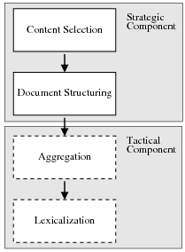
Figure 1.3 shows my assumed two-stage NLG architecture. The Strategic Component is divided into the two modules I am learning. The figure also highlights the interaction between Strategic Generation and both aggregation and lexicalization in the Tactical Component, as they pose challenges to my learning system. The aggregation module will take a list of aggregation chunks (each containing a number of messages) and produce as output a list of sentences (each sentence containing one or more messages). The lexicalization module changes messages into words; it encompasses referring expressions, lexicalization and surface realization. Therefore, aggregation and lexicalization will re-order messages locally; when observing text as evidence of document plans the original ordering will be distorted. I will now discuss Content Selection and Document Structuring as they are the focus of this dissertation.
The Content Selection module takes the full knowledge base as input and produces a projection (a subset) as output. This module should also consider the communicative goal when building the output subset. The output of the Content Selection module has been termed the relevant knowledge pool (McKeown, 1985), viewpoints (Acker and Porter, 1994) or generic structure potential (Bateman and Teich, 1995).
A possible implementation of a Content Selection module uses rules to decide whether
or not to include a piece of information. This decision is based solely on the semantics of the
data (e.g., the relation of the information to other data in the input). These rules take as
input a node in the knowledge representation graph and execute a predicate on it
(f : node → ).
).
The decision of whether to include a given piece of data is done solely on the given data (no text is available during generation, as the generation process is creating the output text).7 The current node and all surrounding information are useful to decide whether or not to include a piece of data. For example, to decide whether or not to include the name of a movie, whether the movie was the reason behind an award (and the award itself) may be of use. Such a situation can be addressed with the rules defined below.
While I experimented with a number of rule languages, I will describe here the tri-partite rule language, a solution that exhibits the right degree of simplicity and expressive power to capture my training material in the biographical profiles domain. Other domains may require a more complex rule language but, in practice, the tri-partite rules are quite expressive and very amenable for learning.
Tri-partite rules select a given node given constraints on the node itself and a second
node, at the end of a path rooted on the current node. For the constraints on nodes, I have used
two particular type of constraints: whether or not the value of the node belongs to a particular
set (e.g., value ∈ ) or a special (True) constraint that
always selects the item for inclusion (the absence of any rule that selects a node
is equivalent to a False rule). Again, more complex constraints are possible, but
these types of constraints are easily learnable. Some example rules are detailed in
Figure 1.4.
) or a special (True) constraint that
always selects the item for inclusion (the absence of any rule that selects a node
is equivalent to a False rule). Again, more complex constraints are possible, but
these types of constraints are easily learnable. Some example rules are detailed in
Figure 1.4.
 (-, -, -). ;Select-All
Always say the first name of the person being described.
 : (false, -, -). ;Select-None
Never say the eye color of the person being described.
 : (value ∈
 , -,-).
Only mention the name of an award if it is whether a Golden Globe or an Oscar.
 : (-,
: (-, ,value ∈
 ).
).
Only mention the title of a movie if the movie received an Oscar or a Golden Globe.
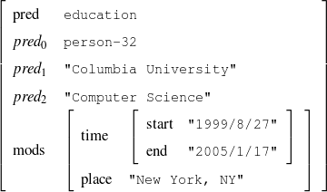
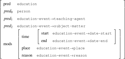
A schema is a particular solution to the Document Structuring task, a task that takes as input a subset of the knowledge base (the relevant knowledge pool) and returns a sequence of messages (a document plan). These messages are produced by communicative predicates (Figure 1.5) composed of three items: variables, properties and output. Each variable has a type, which further constrains the possible values it can take. The actual number and nature of these predicates varies from domain to domain. A predicate can be considered as a function that takes a number of defined (and maybe undefined) variables and searches the knowledge representation for values of the undefined variables that satisfy the constraints inside the predicate. If none are found (or if the provided variables do not satisfy the constraints), the predicate cannot be instantiated. For each set of values8 that satisfy its constraints, the predicate produces a message (Figure 1.6), a data structure assembled using the variable assignment found during the search. The messages are the nexus between the schema and the rest of the NLG system. A predicate, therefore, can be thought of in this context as a blueprint for making messages.
| person | : | c-person |
| education-event | : | c-education-event |

Given a set of predicates, a schema (shown in Chapter 5, Figure 5.3) is a finite state machine over the language of predicates with variable references. At each step during schema instantiation, a current node is kept and all the predicates in the edges departing from the current node are instantiated. A focus mechanism will then select the next node (and add the message to the document plan). The instantiation process finishes when no new predicate can be instantiated departing from the current node. While the schema itself is simple (an automaton with predicate and variable names on its edges), the instantiation process presents some complexities. Interestingly, my schema induction algorithm is independent of the instantiation process or its internal details. However, this complexity forbids using existing learning techniques for finite state machines to learn the schemata.
Schemata are explained in detail in Chapter 2 (McKeown’s original definition, Section 2.2.1) and Chapter 5 (my schemata implementation, Section 5.1).
My research hypothesis is three-fold. First, I share (McKeown, 1983)’s original research hypothesis that the text structure is usually different from the knowledge structure.9 I refer to the structure of the knowledge as domain orderings, such as time or space. This type of information controls some of the placement of information in the text, e.g., news articles about a certain event enumerate some events chronologically (Barzilay et al., 2001). However, these orderings cannot be expected a priori for every domain and, in general, text structure is not governed by them.
Second, as this dissertation focuses on learning schemata, my main hypothesis is centered on the feasibility of automatically constructing schemata from indirect observations, using shallow methods. Indirect observations refer to learning schemata from positive examples, contained in a Text-Knowledge corpus. I have this corpus instead of a fully supervised training material (in the form of document plans or sequences of predicates). Text has a linear structure, defined by the fact that words come one after another. Even though exact word placement is misleading (as it interacts with aggregation and lexicalization), I can match text and knowledge and migrate the text linear structure to the knowledge. In that sense, my hypothesis implies that shallow text analysis methods can be used to acquire Domain Communicative Knowledge (cf. Section 2.2, Chapter 2) for schema construction. That is, to gain information about the domain behavior in general, via Indirect Supervised Learning as described in the next section. This level of analysis lets me gain information about the behavior of the domain in general, but not necessarily solve an understanding task for each particular text.
Finally, part of my research hypothesis is that schemata are useful as a learning representation. Their simplicity, a fact that has been criticized in the literature (Zock, 1986, Hovy, 1993), make them a prime candidate for learning. Moreover, the fact they are learnable should shed more light on their empirical importance (already highlighted by the number of deployed NLG systems employing them (Paris, 1987, Maybury, 1988, Bateman and Teich, 1995, Lester and Porter, 1997, Milosavljevic, 1999)).10
The input to my learning system is thus knowledge and text. For the task of learning Strategic Generation logic, this is a supervised setting; the learning system is presented with the input to Strategic Generation (knowledge) and text that is determined from the output of the strategic generation component (relevant knowledge and document plans). As the text is not the output of the Strategic Generation component, but something that can be derived from the output of the strategic component, my solution to this problem is Indirect Supervised Learning, which I explain at length in Chapter 3, Section 3.2.
As mentioned in Section 1.1, the output of the Strategic Generation component is defined as follows: the relevant knowledge pool is a subset of the knowledge base, which I assume is a frame-based knowledge representation. The document plan is a sequence of messages (rhetorical predicates instantiated from the relevant knowledge pool), segmented into paragraphs and aggregation sets.11
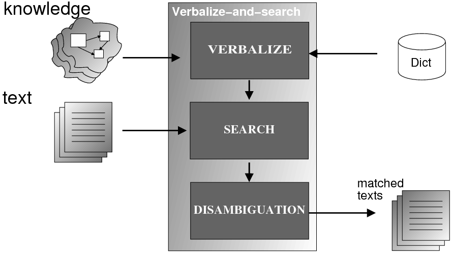
To obtain the relevant knowledge pool and the document plan, I build without human intervention an intermediate structure, the matched text, by using assumptions on how knowledge can be verbalized within the text. These matched texts are built without any examples of actual matched texts (unsupervised learning). For example, the first sentence of the biography in Figure 1.1 will produce the following matched text12 when matched against the knowledge base shown in the figure:
name-first(person-1,'Sean')name-last(person-1,'Connery') is an occupation(person-1,c-actor) and a occupation(person-1,c-producer)
With the matched text in hand, it is easy to see which knowledge has been selected for inclusion in the text: any piece of knowledge matched to a text segment is thus assumed to be selected by the human author for inclusion in the text. Having now a task (Content Selection) with training input (KB) and output (KB plus selection labels) pairs, this comprises a well defined learning problem, where Content Selection rules can be learned.
Continuing with the example, let’s suppose we have two biographies:
The first biography is a business-style biography, while the second one is a family-style biography. For each style, the matched text provides labels for each fact in the knowledge base. These labels (selected or omitted) are shown in Figure 1.7 for the business-style biography.
|
To choose among the different possible rulesets (e.g., ruleset  1 and ruleset 2), I look
at the information retrieval task of retrieving the labels (selected, omitted) for each piece of
knowledge in the input knowledge base. The F*-measure from information retrieval (van
Rijsbergen, 1979) of this retrieval task can be used as a likelihood for each ruleset. The
supervised learning step becomes searching for the ruleset that maximizes this likelihood.
Therefore, if the F*-measure of the labels obtained by applying 1 to the training set
is greater than the F*-measure of applying 2, then 1 should be preferred over
2.
1 and ruleset 2), I look
at the information retrieval task of retrieving the labels (selected, omitted) for each piece of
knowledge in the input knowledge base. The F*-measure from information retrieval (van
Rijsbergen, 1979) of this retrieval task can be used as a likelihood for each ruleset. The
supervised learning step becomes searching for the ruleset that maximizes this likelihood.
Therefore, if the F*-measure of the labels obtained by applying 1 to the training set
is greater than the F*-measure of applying 2, then 1 should be preferred over
2.
The matched text also provides input and output for learning schemata: the input to a schemata-based strategic component is the relevant knowledge pool, extracted in the previous Content Selection step. The output of the schema, the document plan, can not directly be extracted from the matched text, but the sequence of matched pieces of knowledge can approximate the messages.
That is, the sequence of pieces of knowledge (facts) extracted for the matched text of the biography shown in Figure 1.1 will read as follows:
[ name-first(person-1) name-last(person-1) occupation(person-1)
occupation(person-1) ] [ ex-spouse(person-1) name-first(person-2)
name-last(person-2,) occupation(person-2) relative(person-2)
name-first(person-3) ] [ spouse(person-1) name-first(person-4)
name-last(person-4) occupation(person-4) ] [ work(person-1)
title(bond-1) reason(oscar-1) award(person-1) title(oscar-1)
sub-title(oscar-1) ]
Compare this to the document plan shown in Figure 1.1. As document plans are at the
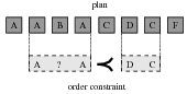
predicate level, I mine patterns over the placement of atomic pieces of knowledge in
the knowledge sequence extracted from the text (in the example above, I find that
 name-first, name-last, occupation
 is a recurring pattern), mine order constraints
over them and use the constraints to evaluate the quality of document plans from
possible schemata. Finally, to compare sequences of atomic pieces of knowledge to
predicates, I defined a dynamic programming-based metric, explained in Chapter 5,
Section 5.4.2.
is a recurring pattern), mine order constraints
over them and use the constraints to evaluate the quality of document plans from
possible schemata. Finally, to compare sequences of atomic pieces of knowledge to
predicates, I defined a dynamic programming-based metric, explained in Chapter 5,
Section 5.4.2.
Given a set of relevant knowledge pool–document plan pairs, I define the likelihood of a schema by summing up three terms:
As with Content Selection, defining means to tell good schemata from bad ones renders the learning problem an optimization one.
On technical grounds, Figure 1.8 shows a generalized graphical model13 for my system. There, my observed input (knowledge base) and output (text) are marked in black. The mapping I am interested in learning is “knowledge base” to “relevant knowledge pool” and “relevant knowledge pool” to document plan.
Indirect Supervised Learning involves an unsupervised step, based on assumptions on the structure
of the model, to elucidate the hidden variables and supervised steps to generalize from the constructed
mapping.14
The assumptions on the model I use are related to the ways knowledge can appear on the text.
More specifically, I see the knowledge as a collection of atomic items (the concepts), and I see
the text as a collection of phrases. The relation between phrases and concepts is given by a
verbalization function  from concepts to sets of phrases (possible verbalizations). The model I
use for the unsupervised part is summarized by the following two tests, where H0 is the null
hypothesis, p and c are particular phrases and concepts,
from concepts to sets of phrases (possible verbalizations). The model I
use for the unsupervised part is summarized by the following two tests, where H0 is the null
hypothesis, p and c are particular phrases and concepts,  is the set of phrases that
make a particular text,
is the set of phrases that
make a particular text,  is the set of concepts that make a particular knowledge
representation (where and refer to the same entity) and is the verbalization
dictionary:
is the set of concepts that make a particular knowledge
representation (where and refer to the same entity) and is the verbalization
dictionary:
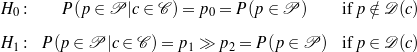
Here, H0 says that if a given phrase p is not a verbalization of a given concept c, then knowing that c holds will not change the chances of p appearing in the text. On the contrary, H1 says that is p is a verbalization for c, knowing that c holds makes it much more likely for p to appear in the text.
Supervised Learning. As the experiments in Chapter 3 will attest, the matched text construction process is able to identify in an automatic fashion training material with an F*-measure as high as 0.70 and as low as 0.53. These results imply that learning using the matched texts as training material will require a robust machine learning methodology. I will now mention some features common to the supervised learning algorithms presented in Chapter 4 and Chapter 5. Both Content Selection rules and Document Structuring schemata are symbolic and highly structured in nature. In both cases, I have input and output pairs (I,O) to learn them, extracted from the matched text. I am interested in finding the object o* (belonging to the set of all possible Content Selection rules or Document Structuring schemata, in either case) such that o* maximizes the posterior probability given the training material:
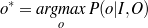
Here, instead of computing the probability P(o|I,O), I use the input/output pairs to compute for each putative object o a likelihood f(o,I,O). This likelihood will also allow me to compare among the different o and it is thus a quality function in the representation space. In both cases, I use a similarly defined function: employ the rules or the schemata to generate from the input I a set of outputs O′. The sought quality function becomes the distance between the training output and the produced output, ||O-O′||, for suitable distances.
Given the quality function, finding o implies a search process on the large space of representations. Several algorithms can be of use here (e.g., A*, hill-climbing or simulated annealing). However, given the highly structured nature of my representations, I have found it valuable to define a successor instance coming from two instances in the search pool, instead of one. This type of approach is known as Genetic Algorithms (GAs). In general, I consider GAs as a meaningful way to perform symbolic learning with statistical methods.
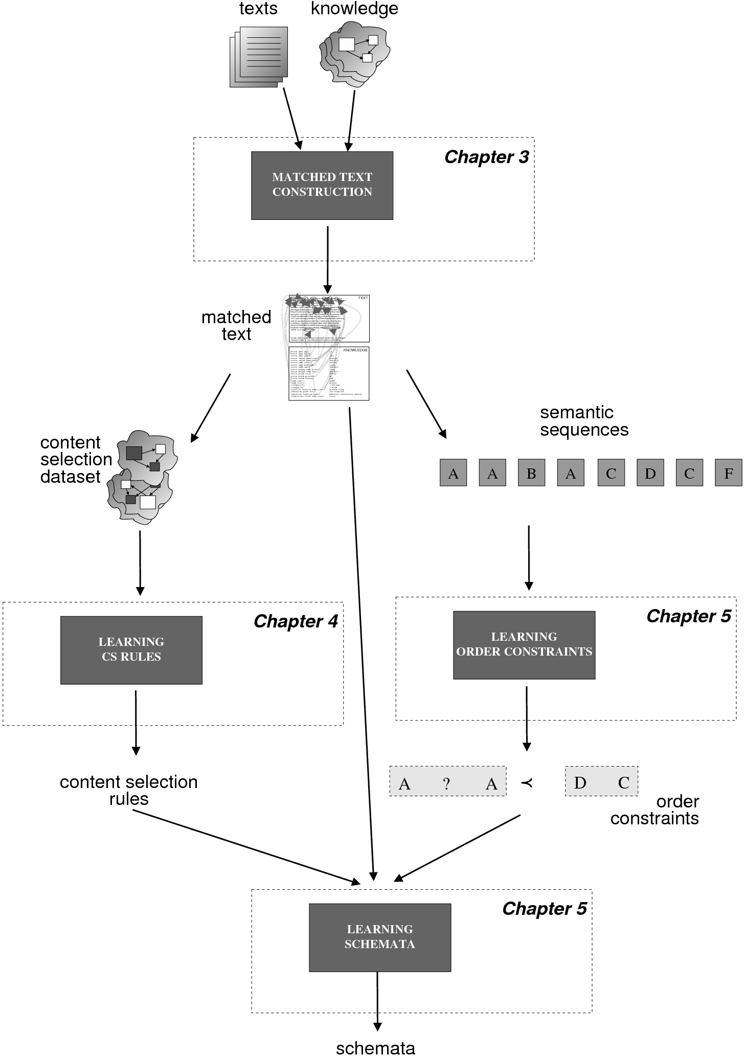
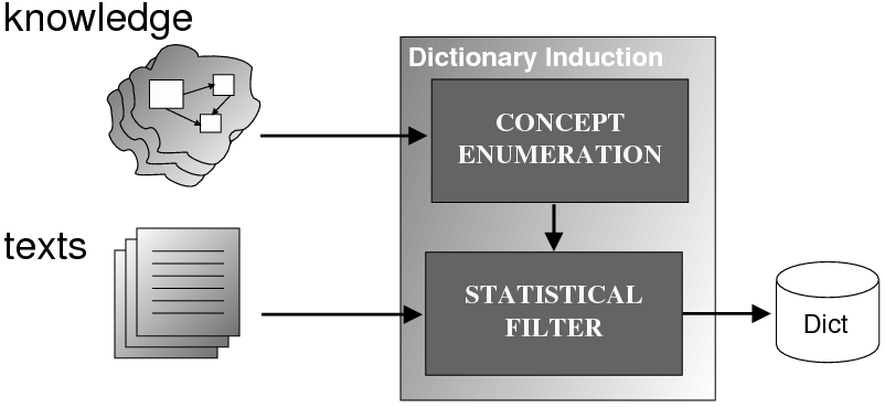
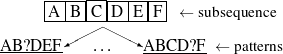
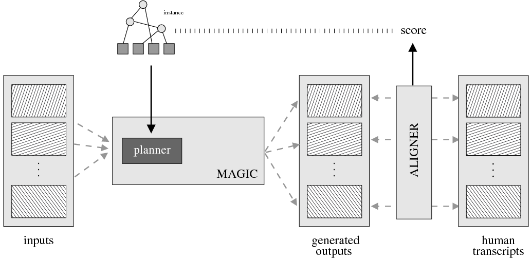
System Architecture. The process described above is sketched in Figure 1.9, using the thresholds and parameters15 described in Table 1.1. The Text and Knowledge corpus is fed into a matched text construction process, described in Chapter 3. This process will employ the model with a minimum score on the t-values (thrt) for concepts that appear in at least thrsupp documents. Once some matches have been identified, a disambiguation process using w words around each match will be spanned.
From the matched text, a Content Selection dataset will be used to learn Content Selection rules (presented in Chapter 4). This process is centered about a GA with a population of populationsize. This initial population is built using a bread-first search until depth depth in the knowledge graph. The fitness function will weight precision and recall using a weight of α.
Also from the matched text, sequences of semantic labels are extracted and used to learn Order Constraints (Chapter 5). For this process, only patterns that appear in a supportthreshold sequences are further considered. The mined constraints are only considered if their associated probability is above throc.
Finally, the Content Selection dataset, the Order Constraints, sequences of atomic values extracted from the matched text and rhetorical predicates are all used to learn schemata (Chapter 5). A population of populationsize(2) is used to learn schemata with a maximum of nv variables per type.
| Threshold | Description | Value |
Chapter 3 | ||
| thrt | t-test cut-point | 9.9 |
| thradd | Percentage of the available number of matches to run
the on-line dictionary induction. | 20% |
| thrtop | Number of top scoring matches to add in each step
(computed as a percentage of the total number of
matches). | 10% |
| w | Disambiguation window, in words. | 3 |
| thrsupp | Concept support, in percentage of the total number of
instances. | 20% |
Chapter 4 | ||
| populationsize | Size of the population in the genetic search for
Content Selection rules. | 1000 |
| depth | Depth cut-off for the breath-first search building the
population for the rule search. | 6 |
| α | F-measure weighting. | 2.0 |
| l | Saturation area of the MDL sigmoid function. | 0.99 |
Chapter 5 | ||
| support threshold | Minimum number of sequences a pattern should
match to be further considered (this threshold is
expressed as percentage of the total number of
sequences). | 30% |
| throc | Probability threshold for a given order constraint to
be further considered. | 0.98 |
| nv | Number of variables per type. | 2 |
| windowsize | How many items are used to build a pattern. | 8 |
relative distance
threshold | Clustering parameter when mining order constraints. | 0.1 |
probability
cut-point | Minimum probability for accepting a learned
constraint. | 0.99 |
This thesis puts forward contributions at three levels. First, it contributes by devising, implementing and testing a system for the automatic construction of training material for learning Content Selection and Document Structuring logic. The technique described in Chapter 3 is able to process hundreds of text and knowledge pairs and produce Content Selection training material with quality as high as 74% precision and 67% recall. The Document Structuring material (orderings) it produces is also highly correlated to hand annotated material. This matched texts construction process emphasizes the use of structured knowledge as a replacement for manual tagging. The Text-Knowledge corpus in the biographies domain assembled as part of this thesis is now a valuable resource, available for further research in the area, together with the machinery to obtain new training material in a number of domains discussed in Chapter 9. The evaluation methodology employed in this thesis is also a contribution: using a number of human written texts for evaluation, dividing them into training and test set and using the test set to evaluate both the unsupervised as well as the supervised steps. Alternative approaches will require larger amounts of human-annotated data or will leave the unsupervised part without proper evaluation.
Second, among my contributions are also the proposal and study of techniques to learn Content Selection logic from a training material consisting of structured knowledge and selection labels. As the training material is automatically obtained, it contains a high degree of noise. Here, my contribution includes techniques that are robust enough to learn in spite of this noise. I set the problem as a rule optimization of the F*-measure over the training material. My techniques have elucidated Content Selection rules in four different styles in the biographies domain. Moreover, my experiments in Content Selection contribute to our understanding of the Content Selection phenomenon at several levels. First, it separates nicely the need for off-line (high-level) Content Selection from on-line Content Selection, where the approach described in this thesis could potentially be used to learn Content Selection logic at both levels.16 From a broader perspective, my acquired Content Selection rules provide an empirical metric for interestingness of given facts.
Finally, I defined the problem of learning Document Structuring schemata from indirect observations, proposing, implementing and evaluating two different, yet similar techniques in two different domains. The Document Structuring problem is one of the most complex problems in NLG. My techniques are among the first efforts to effectively learn Document Structuring solutions automatically. At a fine grained level of detail, my main contribution is a dynamic-programming metric that compares sequences of values (that can be read out from text) to sequences of messages (that are produced by the schemata). The acquired schemata are written in a declarative formalism, another contribution of this thesis. Previous implementations of schemata had mixed declarative/procedural definitions that impose a high burden for any learning technique.
I discuss now my experimental domains (Medical Reports and Person Descriptions). These domains were central to research projects I have been involved with. Other potential domains are discussed in Section 9.3, including Biology, Financial Markets, Geographic Information Systems, and Role Playing Games.
MAGIC (Dalal et al., 1996, McKeown et al., 2000) is a system designed to produce a briefing of patient status after the patient undergoes a coronary bypass operation. Currently, when a patient is brought to the intensive care unit (ICU) after surgery, one of the residents who was present in the operating room gives a briefing to the ICU nurses and residents. The generation system uses data collected from the machine in the operating room to generate such a presentation, avoiding distracting a caregiver at a time when they are critically needed for patient care.
Figure 1.10 shows an example of a data excerpt (a data file in the classic formalism with 127 facts on average) and presentation. Several of the resident briefings were collected and annotated for a past evaluation. Each transcription was subsequently annotated with semantic tags as shown in Figure 6.2, on page §.
| Input Knowledge | MAGIC output |
(patient-info-12865, c-patient, (a-age,
age-12865), (a-name, name-12865), (a-gender,
gender-12865), (a-procedure, procedure-12865),
(a-birth-date, …), …)
(age-12865, c-measurement, (a-value, 58), (a-unit, "year")) (gender-12865, c-male) (ht-12865, c-measurement, (a-value, 175), (a-unitm "centimeter")) (name-12865, c-name, (a-first-name, "John"), (a-last-name, "Doe")) (procedure-12865, c-procedure, (a-value, "mitral valve replacement")) … | John Doe is a 58 year-old male patient
of Dr. Smith undergoing mitral valve
repair. His weight is 92 kilograms and his
height 175 centimeters. Drips in protocol
concentrations include Dobutamine,
Nitroglycerine and Levophed. He received
1000 mg of Vancomycin and … |
As part of the Question Answering project (AQUAINT) taking place jointly at Columbia University and University of Colorado, I have developed ProGenIE, a system that generates biographic descriptions of persons, taking as input information gathered from the WWW. The biographical descriptions domain is central, as it has available larger amounts of data compared to the medical domain. Because of this data availability, I only pursued Content Selection experiments in this domain.
For these experiments, fact-sheet pages and other structured data sources provide the input knowledge base (Duboue and McKeown, 2003b). The texts are the biographies written by professional writers or volunteers, depending on the corpus. Figure 1.11 exemplifies an aligned pair.
This domain is very rich, allowing me to gather multiple biographies for each person I have independently obtained knowledge. Such multi-aligned corpus had also proven useful for mining verbalization templates (Barzilay and Lee, 2002).
| Input Knowledge | Human-written Text |
fact(person42,name,'Sean Connery').
fact(person42,birthname,'Thomas Sean Connery'). fact(person42,birthdate,month('August'),day('25'), fact(person42,birthplace,'Edinburgh, Scotland'). fact(person42,education,'Dropped out of school at age 13'). fact(person42,family,Mother,name('Euphamia Connery')). fact(person42,family,Brother,name('Neil')). fact(person42,family,Son,name('Jason Joseph Connery')). fact(person42, occupation, "actor"). fact(person42, occupation, "director"). fact(person42, occupation, "model"). fact(person42, occupation, "producer"). … | Actor, born Thomas Connery on August
25, 1930, in Fountainbridge, Edinburgh,
Scotland, the son of a truck driver and
charwoman. He has a brother, Neil, born
in 1938. Connery dropped out of school
at age fifteen to join the British Navy.
Connery is best known for his portrayal of
the suave, sophisticated British spy, James
Bond, in the 1960s. … |
This dissertation is divided into the following chapters.
In this chapter, I discuss related work in Strategic Generation and learning in NLG. These topics are very broad; I have decided to focus on a small number of highly relevant papers. I first analyze related work in Content Selection (Section 2.1), in particular, the work on the ILEX (Cox et al., 1999, O’Donnell et al., 2001) and STOP (Reiter et al., 1997) projects. Afterwards, I introduce the Document Structuring task together with schemata and RST, its two most widespread document structuring solutions. I then relate my work to other recent learning efforts in NLG in Section 2.3. To conclude this chapter, I present related work in a number of assorted areas, including the relation between the strategic component and other modules of the NLG pipeline, planning diverse media, summarization and biography generation.
Content Selection, the task of choosing the right information to communicate in the output of a NLG system, has been argued to be the most important task from a user’s standpoint; users may tolerate errors in wording, as long as the information being sought is present in the text (Sripada et al., 2001). This task has different levels of complexity, with solutions requiring a full inferential engine in certain cases (Zukerman et al., 1996).
I will present here one of the most recent Content Selection algorithms in the literature, developed as part of the ILEX project and compare it to my two level Content Selection approach. In Section 2.1.2, I will summarize the knowledge acquisition process that the researchers in the STOP project pursued to build their Content Selection module. I will also compare that human acquisition with my the automated one described in Chapter 4. Some remarks regarding integrated or separated Content Selection close this section.
One of the most well-regarded integrated Content Selection algorithms proposed in the literature is the one used in the ILEX project (Cox et al., 1999, O’Donnell et al., 2001), a generation system that provides dynamic labels for exhibits in a Web-based museum gallery. ILEX tries to improve current static (fully pre-written) Web pages by means of Dynamic Hypertext (Dale et al., 1998), the marriage of NLG and hypertext systems. In Dynamic Hypertext, a generator will produce not only text that lives in the nodes of a hyper-linked environment, but also the links between these nodes.
In the ILEX Content Selection algorithm, each tuple coming from a relational database is transformed into an object definition where each of the entries in the object must be declared in a predicate definition (Figure 2.1). These definitions contain, among other things, a simplified user model composed of three items: interest (how appealing is this fact to the user, static), importance (contribution of the fact for an overall task, also static) and assimilation (level of acquaintance to the fact, dynamically updated). These numbers are hardwired in the predicate definition.
Their algorithm computes a relevant knowledge pool with an innovative relevancy metric. They follow the same line of work presented by (McKeown, 1985) Content Selection (pages 113–121, “Selection of relevant knowledge”), that is, to take the object being described and the entities directly reachable in the Content Potential, a graph with objects as nodes. ILEX also collects all entities relevant to the entity being described, with an innovative spreading-activation relevancy metric. In this metric, the relevancy of an object is given by the mathematical combination of the static importance of the object and the relevancy of the object in the path to the object being described. Their relevance calculation allows them to prioritize the top n most salient items, while maintaining coherence. Different links preserve relevance in different ways. ILEX authors assigned for each class of links hand-picked relevancy multipliers.
The ILEX Content Selection algorithm is complementary to my approach. For instance, my algorithm could be used to provide ILEX interest scores, an appealing topic for further work.
(Reiter et al., 1997)’s work addresses the rarely studied problem of knowledge acquisition for Content Selection in generation. Knowledge acquisition is used for STOP, a NLG system that generates letters encouraging people to stop smoking. STOP’s input is a questionnaire, filled out by a smoker; STOP uses the questionnaire to produce a personalized letter encouraging the smoker to quit. Reiter et al. explored four different knowledge acquisition techniques: directly asking experts for knowledge, creating and analyzing a corpus, structured group discussions and think aloud sessions. I detail each of them below.
The first technique they employed was to directly inquire domain experts for Content Selection knowledge, given that STOP was a multidisciplinary project with motivated experts within reach of the NLG team. This technique proved unsuccessful, as experts would usually provide “textbook style” responses (academic knowledge). Such knowledge differs very much from their actual knowledge as practitioners.
Their next effort focused on creating a small Text-Knowledge corpora (what they call a conventional corpus). They collected 11 questionnaire-letter pairs, with letters written by five different experts. Problems arised when comparing letters written by different doctors; the difference in style, length and content make this corpus very difficult to use.
Their final two methods were borrowed from the Knowledge Engineering literature (Buchanan and Wilkins, 1993) and proved to be very useful (structured group discussions and think-aloud sessions).
This research is relevant to my Content Selection work (presented in Chapter 4) where I propose automated mining of Content Selection rules from a Text-Knowledge corpus similar to the one Reiter et al. collected. Interestingly enough, they found the corpus approach insufficient. I find these possible explanations to their problem:
These problems are not present in my biographies work (neither in a number of domains that I have identified as suitable for application of my technique), where I have found hundreds of biography-knowledge pairs, written by professional biographers that have to adhere to a writing style.
While most classical approaches (Moore and Swartout, 1991, Moore and Paris, 1993) tend to perform the Content Selection task integrated with the Document Structuring, there seems to exist some momentum in the literature for a two-level Content Selection process (Lester and Porter, 1997, Sripada et al., 2001, Bontcheva and Wilks, 2001). For instance, (Lester and Porter, 1997) distinguish two levels of content determination: local content determination is the “selection of relatively small knowledge structures, each of which will be used to generate one or two sentences,” while global content determination is “the process of deciding which of these structures to include in an explanation.” Global content determination makes use of the concept of viewpoints, introduced by (Acker and Porter, 1994), which allow the generation process to be somewhat detached from the knowledge base (KB). My Content Selection rules, then, can be thought of as picking the global Content Selection items.
In the same vein, (Bontcheva and Wilks, 2001) use a Content Selection algorithm that operates at early stages of the generation process, allowing for further refinement down the pipeline. They present it as an example of techniques to overcome the identified problems in pipelined architectures for generation (they call this a recursive pipeline architecture, similar to (Reiter, 2000)).
Most recently, the interest in automatic, bottom-up content planners has put forth a simplified view where the information is entirely selected before the document structuring process begins (Marcu, 1997, Karamanis and Manurung, 2002, Dimitromanolaki and Androutsopoulos, 2003). While this approach is less flexible, it has important ramifications for machine learning, as the resulting algorithm can be made simpler and more amenable to learning. Nevertheless, two-level Content Selection can provide a broad restriction of the information to consider, with more fine grained, hand-built algorithms applied later on to select information in context or with length restrictions.
My work is in the schema tradition, with a two level Content Selection. The first, global level is performed with Content Selection rules and the second level is within the Document Structuring schema.
I will now address some generalities to the Document Structuring problem; namely, its output and overall algorithms employed, before introducing schemata and RST-based planners, the two most widely deployed solutions.
The output of the Document Structuring is a document plan, normally a tree or a sequence of messages. The relations between these messages usually are rhetorical in nature and employed later on to divide the discourse into textual units, such as paragraphs or bulleted lists (Bouayad-Agha et al., 2000) and sentences (Shaw, 2001, Cheng and Mellish, 2000). Most systems use trees as document plans; the RAGS consensus architecture (Cahill et al., 2000) defines the Rhetoric representation level as a tree. Sequences, on the other hand, are more restricted than trees, but for several applications present enough expressive power. Examples include the works of (Huang, 1994) and (Mellish et al., 1998). Sequences are important for my work as schemata, as defined originally by (McKeown, 1985), use sequences as document plans (when employed without schemata recursion). Moreover, even if trees have more momentum as document plans in the literature, several incompatibility results (Marcu et al., 2000, Bouayad-Agha et al., 2000), may suggest otherwise. The use of trees seem forced in some cases, for example (Mann and Thompson, 1988) claim that the rhetorical structure ought to be a tree in most of the texts. However, their Joint rhetorical relation seems to be just an ad hoc procedure to keep a tree from becoming a forest (Rambow, 1999). Finally, (Danlos et al., 2001) analyze cases where trees are not expressive enough. Their solution is to employ equational systems (actually directed acyclic graphs or DAGs) that increase expressivity by reusing rhetorical nodes.
The algorithm normally involves a search on the space of possible document plans. That is the case of Schemata-based, RST-based or opportunistic planners, which I discuss later in this section. However, several Document Structuring problems in the literature have been solved with no search, as in a good number of cases, planning is just a label for a stage solved by other means, as pointed out by (Rambow, 1999). Complex planning process examples include (Huang, 1994), working on automatic verbalization of the output of theorem provers and (Ansari and Hirst, 1998), working on generating instructional texts. In general, full planning is the most comprehensive solution to the document structuring problem, although it is expensive and requires modeling complex issues such as the intentional status of both hearer and speaker, and the full consequences of all actions that may not be necessary (or even feasible) in all domains of interest to NLG practitioners.
Another question being asked by previous research is the direction of the building of the plan. Normally, speed and ease of understanding motivates building top-down planners, e.g., (Young and Moore, 1994), which uses the Longbow AI planner (Young, 1996). However, other authors, for example (Marcu, 1997), see the whole planning process as a linking among facts by means of input-given RST-relations, an approach that is indeed bottom-up (I discuss opportunistic planners in Section 2.2.2). A hybrid approach is taken by (Huang, 1994), which combines a top-down (planned) approach with a bottom-up opportunistic perspective based on centering.
Several other approaches have been investigated. Besides the approaches I discuss later in this section, (Power, 2000) poses the problem as a constraint satisfaction and uses CSP techniques (Jaffar and Lassez, 1986) to solve it. (Knott et al., 1997) make a stand for the use of defeasible rules as a tool for planning coherent and concise texts. (Wolz, 1990) models the problems by having different AI-plans compete with each other to come out with a final decision (another mechanism for doing CSP). In my work, I learned schemata from data (a bottom-up approach), where the schemata are a type of planner that involves a local search during instantiation (top-down skeleton planners, as discussed by (Lim, 1992)).
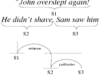
Traditionally, Strategic Generation problems have been addressed in NLG by means of two techniques: AI planners and Schemata. Reasoning can derive the text structure in some cases. In a scenario (Figure 2.2) borrowed from the work of (Rambow, 1999), a reasoning process 1 can derive the text shown in the figure, using, for example, operators derived from rhetorical relations (Section 2.2.2). Reasoning-based Strategic Generation focuses on domains where the structure can be fully deduced from the input data and the intentions of the speaker.
Not all text can be fully deduced from the input; some text has fixed structure coming from the domain. Even though I consider AI-style content planning a useful and interesting approach, many cases require special domain knowledge. For instance, if I know that an actor won three Oscars, was married twice and is 58 years old, common knowledge about biographies would dictate starting a biography with the age and occupation, leaving the rest of the information for later. Nothing intrinsic to age or awards specifies this ordering (it is not part of the domain knowledge itself). The text structure in formulaic domains presents very little intentional structure and is historically motivated; while its current form has logically evolved over time, there is no rationale behind it that can be used for planning. What is needed in such domains is domain knowledge related to its communicative aspects: Domain Communication Knowledge (DCK). DCK has been defined by (Kittredge et al., 1991) as:
(…) the means of relating domain knowledge to all aspects of verbal communication, including communicative goals and function. DCK is necessarily domain dependent. However, it is not the same as domain knowledge; it is not needed to reason about the domain, it is needed to communicate about the domain.
This knowledge can be explicitly or implicitly represented in a strategic component, depending on the judgement of the authors and on its importance for the scenario at hand. In most cases it is left implicitly represented. A notable exception is the work of (Huang, 1994), which defines the notion of proof communicative act (PCAs).
|
 |
What is happening behind the scenes is that three different structures can be mapped to the discourse: informative, intentional and focus. In certain domains, one structure dominates the production of texts and a formalism based on only one of them can be enough to structure the text. (Rambow, 1999) proposes an integrated approach to deal with DCK and other issues.
With respect to intention, (Moore and Paris, 1993) (also (Hovy, 1988)) present a discussion of how to represent the beliefs of the Hearer and the intentions of the Speaker in instructional dialogs. Also, the degree of belief may be important to model as in the works of (Zukerman et al., 1996), (Walker and Rambow, 1994) and (Rambow, 1999). However, other approaches, e.g., (Moore and Paris, 1993) and (Young and Moore, 1994), prefer to consider belief as a binary (believe or disbelieve) datum. In my work, I do not represent nor use intentional structure, beyond the Report(Fact) type of intention, as part of simplifying assumptions to make Strategic Generation amenable for learning. An interesting area for future work is to incorporate intentional data coming from text by using current research in opinion identification (Zhou et al., 2003, Yu and Hatzivassiloglou, 2003). The matched text can be enriched with opinion and opinion polarity labels by an automatic opinion/polarity tagger. My system can then use this extra information to theorize Content Selection rules that take into account the agent’s stance toward certain facts (that information will need to be modelled outside of the learning system, using traditional cognitive modelling).
I will turn now to schemata-based document structuring.
In this section, I present McKeown’s original schemata, then discuss KNIGHT, MAGIC and other schema-like systems. McKeown’s schemata are grammars with terminals in a language of rhetorical predicates, discussed below. The four schemata identified by McKeown in her work are the attributive, (Figure 2.3) identification, constituency, and compare and contrast schemata. The schemata accept recursion, as some entries inside the schema definition can be fulfilled directly with predicates or by other schemata. They are not fully recursive as only four schemata are proposed and there are 23 predicates, although McKeown expressed her belief that the formalism can be possibly extended to full recursion.
| Attributive Schema |
Attributive {Amplification; Restriction} Particular-illustration* {Representative} {Question; Problem; Answer} / {Comparison; Contrast; Adversative} Amplification/Explanation/Inference/Comparison |
Her predicates are important for my work as they contain a major operational part, the search for associated knowledge. When the schema reaches a rhetorical predicate such as attribute, it fills it with required arguments, e.g., the entity the attribute belongs to. From there, the rhetorical predicate (actually a piece of Lisp code) will perform a search on the relevant knowledge pool for all possible attributes to the given entity. These instantiated predicates (messages in this dissertation) will be available for the schema-instantiation mechanism to choose (by virtue of her focus mechanism, explained below) and then build the document plan.
Schemata are then structure and predicates. My work focuses in learning the structure but not the predicates (I basically learn only part of the schemata, in a sense). Which predicates to use and how to define them is an important part of the schema that I thus assume to be part of the input to my learning system. This is a point of divergence with McKeown’s schemata that used predicates rhetorical in nature. My predicates are domain dependent, what makes creating these predicates a process worth automating. As a step in that direction, I have been able to provide a declarative version of these predicates in a constraint satisfaction formalism (discussed in Chapter 5, Section 5.1).
To implement the schemata, McKeown employed Augmented Transition Networks (ATNs) an extensible declarative formalism where some of her requirements used these extensions. In her system, the rhetorical predicates are executed when traversing different arcs. Both the actions in the arcs and the conditions are arbitrary pieces of Lisp code. An example ATN (Figure 2.4) shows a fair degree of possibilities at each node (seen by the number of arcs leaving each state). One contribution from McKeown’s work is to use focus to guide the local decision of which arc to traverse at each moment. I will discuss her focus mechanism now.
(McKeown, 1985) contains a full chapter (“Focusing in Discourse,” pages 55–81) describing the importance of centering theory and proposing a motivated solution for discourse planning. She built on the works of both Grosz (global focus) and Sidner (local focus) to extend their interpretation theories with decision heuristics for generation. McKeown’s work on focus is a major ingredient of her schemata and has been adapted for use in other generation systems (e.g., (Paris, 1987)’s TAILOR generator). However, few schema-like planners mentioned in the literature include this piece of the schema. I find that a major oversight of later followers of McKeown’s work.
As pointed out by (Kibble and Power, 1999), research on focus in understanding is interested in discourse comprehension, mostly solving cases of anaphora, e.g., pronominalization. Most centering theories, therefore, provide tools to cut down the candidate search space for anaphora resolution. Nevertheless, the generation case is different, as these theories lack insights of how to choose among the set of candidates. Understanding does not require these decisions, as they have been taken by the human author in the text already. McKeown complemented centering theories with heuristics suitable for generation. For recent work on centering, (Karamanis, 2003) presents a learning approach to the problem.
McKeown presents heuristics for two decision problems involving focus. In the first problem, the system has to decide between continuing speaking about the current focus or switching to an entity in the previous potential focus list. Her heuristic in that case is to switch, otherwise the speaker will have to reintroduce the element of the potential focus list at a later point. The next decision arises when deciding whether to continue talking about the current focus or switching back to an item in the focus stack. Here her heuristic was to stick to the current focus, to avoid false implication of a finished topic.
This is, grosso modo, McKeown’s treatment of focus. The details are more complex but I will skip them as I use McKeown’s focus mechanism without any modifications. Her focus mechanism is important because my machine learning mechanism interacts with it and has to learn schemata in spite of the actual focus system.
(Lester and Porter, 1997) were interested in robust explanation systems for complex phenomena. When designing their Document Structuring module, they focused on two issues, expressiveness (the Document Structuring module should be able to perform its duties), and Discourse-Knowledge Engineering (DCK requires expertise to be acquired and represented, see Section 2.2, they were particularly interested in providing tools to support this vision). This last issue arise after working in an non-declarative Explanation Planning module for a period of time. As the module grew larger, adding new functionality or understanding existing ones became an issue as the actual logic was buried under lines and lines of Lisp code.
To solve this problem, Lester and Porter took the most declarative pieces of their approach and moved it to the knowledge representation system, creating the Explanation Design Packages (EDP). EDPs are trees represented as frames in a knowledge representation. The frames encapsulate a good deal of Lisp code, defining local variables, conditions over local and global variables, invoking KB accessors and arbitrary functions. They are as rich as a programming language.
When compared to schemata, it seems that Lester and Porter arrive at a similar solution coming from the opposite direction. McKeown analyzed a number of texts and background work in rhetorical predicates to hypothesize her schemata as a suitable representation of discourse that she later operationalized using ATNs. As ATNs are of a hybrid declarative/procedural nature, extensions can be coded in by means of extra Lisp code. Her schemata required using some of these extensions. McKeown, therefore, arrived at a hybrid declarative/procedural implementation starting from a fully declarative problem. Lester and Porter, on the other hand, started with a fully procedural implementation and further structured and simplified it until they arrived to their hybrid declarative/procedural EDPs.
True to their roots, EDPs have a more procedural flavor, but that does not avoid making a direct comparison with schemata. The frames in EDP correlate roughly to schemata’s states. Note, however, that there are no cycles on the EDPs (as they are trees). The loops in the schemata are represented in EDP by an iteration mechanism. More interestingly, the KB accessor functions behave operationally exactly the same as McKeown’s predicates. The major difference (and this may be the reason why Lester and Porter did not draw this parallelism) is that McKeown stressed the rhetorical nature of her predicates. KNIGHT predicates are not rhetorical, but domain dependent; this is an approach I follow in my work as well. Finally, both approaches allow plugging a sizeable amount of extra Lisp code into their formalisms. EDPs provide more places to do so, while the ATNs concentrated this in the arc transitions.
A key distinction is that, while schemata are skeleton-planners because they contain the skeleton of a plan but they perform a local search (driven by McKeown’s focus mechanism) to arrive to the final plan (Lim, 1992), EDPs lack any type of search. Lester and Porter did not mention this fact on their work and it is clear they did not need such a mechanism for their robust generation approach.
EDPs expand schemata by providing a hierarchical organization of the text that is suitable for multi-paragraph texts. Moreover, they include a prioritization model that makes for a bare-bones user model (but does not compare to either the TAILOR (Paris, 1987) or ILEX (O’Donnell et al., 2001) treatment of the issue) and a number of well-defined non-rhetorical predicates for natural entities and processes. However, Lester and Porter followed a more procedural extension of the schemata, which makes them unsuitable for my learning approach.
MAGIC. MAGIC took the topic tree approach of Lester and Porter and simplified it until it became fully declarative, with a high toll on its expressive power. Its schema is a tree with topic internal nodes and predicate-leaves. The internal nodes constitute the text organization and structure the output into two levels of chunking (paragraph chunks that contain aggregation chunks). The predicate-leaves fetch from the knowledge base all the values matching the predicate and insert the resulting messages into the output. This is the only iteration process in the MAGIC planner. By being encapsulated into the leaves, it spares the need of cycles as in TEXT or iterators and local variable definitions as in KNIGHT. The MAGIC planner is so simple that it is surprising that it works. A closer look may reveal MAGIC’s secret: the repetition-at-the-leaves approach produces highly cohesive lists of related facts, realized in the form of enumerations, with the rest of the information shuffled around inside the aggregation chunks by the MAGIC complex aggregation component, one of the foci of the project. Interestingly enough, this representation was very amenable to my learning techniques (Chapter 5). The representation, however, seems only suitable for planning single-topic discourse (all discourse in MAGIC has the same focus —the patient the surgery was about).
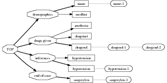
Other schemata implementations. Plenty of other people used schemata, including the work in the TAILOR generator (Paris, 1987) that expands schemata with user model and trace-explanation systems, the work done by (Maybury, 1988) that attempts to add more rhetorical predicates, the work in the KOMET project (Bateman and Teich, 1995) that expands schemata for text and graphics, and the work in the Peba-II system, that applies schemata to dynamic multimedia and comparisons (Milosavljevic, 1999). I detail my own declarative implementation of schemata in Chapter 5.
Continuing with the idea already present in McKeown’s work of consolidating and improving rhetorical relations defined previously in the literature, (Mann and Thompson, 1988) studied a number of texts in different genres and styles and formulated their Rhetorical Structure Theory (RST). RST states that every text has a unique rhetorical structure based on text spans where rhetorical relations hold. They add to the rhetorical treatment of McKeown two key ingredients: hierarchy and asymmetry. Now a text span can be subdivided into sub-relations and a super relation can hold over it. Schema recursion is supposed to capture this fact but McKeown did not investigate schema recursion much herself. Hierarchy is not the only key ingredient added to the picture by Mann and Thompson, as they also realize that a number (almost all) of the rhetorical relations they identified in texts were asymmetrical, in the sense that they contained two text spans, one of which (the nucleus) was central to the discussion and could not be removed, while the second span (the satellite) expands or complements the nucleus.
From their analysis, they propose 23 rhetorical relations, divided into two categories, presentational and informational. The distinction is made depending on whether they hold in the text by virtue of the text flow (presentational) or by virtue of the underlining truth of the given facts (informational). For example, a relation such as Justify will only hold depending on what has been said before and what we want to say now (that is, it depends on the information selected and how it is placed on the text, in the intention of the speaker), while a relation such as Volitional Cause holds statically between two facts in the knowledge base.
RST is a theory designed to capture the structure of texts in general, without particular ties to understanding or generation. Relative early success in understanding (Marcu, 2000) has run into problems defining a set of rhetorical relations (Marcu and Echihabi, 2002). Nowadays, the existence of rhetorical relations that hold between spans of text is an agreed fact and research focuses on the sizes of those spans and the number and nature of the relations. Regarding the size of the spans, (Mann and Thompson, 1988) work at the clause level but other researchers such as (Stent, 2000) use variable sizes from words to sentences. Regarding the number of the relations, (Knott and Dale, 1993) provide a bottom-up perspective on the number of relations issue, postulating that despite the actual relations taxonomy, it should in some way be reflected by the existence of related cue phrases. (Marcu and Echihabi, 2002) put this idea into practice, in their study using a very large corpus. Other approaches postulate a large number of relations, which (Hovy and Maier, 1995) organized in a taxonomy. Finally, there is the issue of whether or not the number of rhetorical relations is bounded. On the one hand, (Rambow, 1999) and (Knott and Dale, 1993) argue in favor of bounding their number as otherwise the theory will become unsound. On the other hand, (Mann and Thompson, 1988) and (Hovy and Maier, 1995) sacrifice soundness on behalf of a further reaching theory (on pragmatic grounds).
From the generation perspective, (Hovy, 1988) was the first to apply it for building a strategic component (Hovy, 1993). His approach involved reversing the direction of the RST relations defined by Mann and Thompson (so its observed effect is used as a precondition and its applicability constraints as post-conditions) and using them as operators in a planning process. While this approach enjoyed limited success, it has a number of drawbacks. Some problems between this planning approach and intentional structure have been discussed at length by (Moore and Pollack, 1992) (e.g., how intentional structure will be lost if only rhetorical structure is kept as the output of the planner, complicating follow-up reasoning over the generated text), but more relevant to my dissertation are the operational issues involved in a RST-based planner. Building a RST-based planner requires modelling carefully the intentions of both the speaker and the hearer (cognitive modelling), a problem in purely informative domains, where the only intentional structure that can be associated with the text is the simple Report(Facts). Moreover, purely informative domains are prime candidates for using NLG techniques and therefore of practical importance. As pointed out by (Lim, 1992), a RST-planner requires additional guidance to be able to plan reasonable text in reasonable amounts of time. In that direction, my work can be adapted to acquire this domain-based information from a Text-Knowledge corpus.
Another avenue to incorporate rhetorical relations when planning purely informative texts is to rely solely on informative relations, precalculated on the semantic input (considered, therefore as an integrated part of the knowledge representation) and then search for a text that is able to incorporate as many of the rhetorical relations as possible (Marcu, 1997), together with other text structuring operators (Mellish et al., 1998) and most importantly, focus-based constraints (Karamanis and Manurung, 2002). That approach renders the document structuring an optimization process, a search for the text structure that maximizes an evaluation (objective) function. Interestingly enough, the techniques employed to solve this problem involve also genetic algorithms (in particular, Genetic Search (Michalewicz, 1992)). I also use genetic algorithms in my work. While (Mellish et al., 1998)’s intention was to push stochastic search as a feasible method for implementing a document structurer, I pursue the automatic construction of the schema itself. My system, moreover, uses a corpus-based fitness function, while they use a rhetorically-motivated heuristic function with hand-tuned parameters.
Considering rhetorical relations as part of the input has the advantage of avoiding an explicit representation of the intentional state of the Hearer. In such settings, a trivial cognitive model, where every fact uttered by the speaker will be immediately assimilated and believed by the hearer, can be employed. While opportunistic planners succeed in incorporating rhetorical relations in their outputs, they seem to be limited to problems lacking any real use of the communicative power of the rhetorical structure. In contrast, most content planners, (Young and Moore, 1994) and architectures (Cahill et al., 2000) find the relations while structuring the document. By doing so, they can find relations that hold as a result of the structure (presentational relations). In my case, the input is the relevant knowledge pool, a subset of the KB in the frame-based Knowledge Representation described in Chapter 1, Section 1.1.1 and it contains no rhetorical information.
In recent years, there has been a surge of interest in empirical methods applied to natural language generation (Columbia, 2001). One of the first applications of machine learning to NLG systems is a hybrid architecture trained on target text (example outputs) introduced by (Knight and Hatzivassiloglou, 1995). In this architecture, a first component over-generates a large number of possible solutions, and a second component chooses among them. The first component is quite simple and the second component is the one based on machine learning. For example, a symbolic engine may generate his success as an actress and her success as an actress but the probabilities in a corpus of related texts will choose the second (correct) output. My system is an example of an alternative architecture that is trained in input/output pairs, in the form of a Text and Knowledge corpus (besides the fact that my system works in learning for the Strategic Generation component and not the syntactic/realization component).
Text-Knowledge corpora, a traditional resource for knowledge acquisition in Natural Language Generation, are recently gaining momentum as a resource for Statistical NLG (Barzilay and Lee, 2002, Duboue and McKeown, 2002, Sripada et al., 2003, Barzilay et al., 2003). They have been employed for learning elements at the strategic level (Duboue and McKeown, 2002, Duboue and McKeown, 2003a), for lexical choice (Barzilay and Lee, 2002, Sripada et al., 2003) and at other levels (Barzilay et al., 2003, Ratnaparkhi, 2000).
(Dimitromanolaki and Androutsopoulos, 2003) worked also in machine learning applied to Document Structuring. Their training material consisted of sequences of atomic values, an ideal training set, as each atomic value was actually a message and thus the input of the document structurer was compatible with its output. In my case, in contrast, the input are facts and the output are messages assembled over those facts. Because each of these sequences was rather short (about six messages long), the following approach proved fruitful: they trained a cascade of classifiers to decide the exact (absolute) position that each pre-selected fact has to take in the output. It is unclear whether their approach will apply to other (more complex) settings. Absolute and relative positioning are quite similar in sequences of six elements, but in longer sequences, telling between the two allows for a better utilization of the training material. My mining of order constraints described in Chapter 5 is an example of relative orderings.
(Shaw and Hatzivassiloglou, 1999) work on the probabilistic ordering of pre-modifiers in complex NPs (e.g., “a 35-year-old asthmatic male patient of Dr. Smith”), a task also addressed by a number of authors (Cheng et al., 2001, Malouf, 2000, Poesio et al., 1999). Because this type of ordering information is domain dependent, they designed an algorithm to acquire order constraints from a corpus. This algorithm is important for this thesis, as I have employed an adaptation of it for my Document Structuring work described in Chapter 5. Their algorithm starts by collecting a table of observed ordering behaviors. In this table, the entry at position i,j indicates the number of times in the corpus the object i came before the object j. From the table, they try to reject the null hypothesis that i,j came in any order (equivalent to saying that the probability of i coming before j is 0.5). The following formula will compute the probability of the observed frequencies:

where m is the total number of times i has been seen occurring before j in the corpus and n is total number of times i and j occur in a pair. That equation can be used with a threshold to select “likely enough” constraints or can be piped into more complex, smoothing techniques described at length by (Shaw, 2001).
Nitrogen (Langkilde and Knight, 1998) is the generation component in a Japanese-English machine translation system. They employ a language model like those used in speech recognition (an n-gram model, in this case a bigram model) and a symbolic module that uses a grammar to transform the input representation into an intermediate representation (a word lattice) that is scored by the language model. The word lattice has several drawbacks (Langkilde and Knight, 1998). Langkilde (Langkilde, 2000) moves away from the word lattice by replacing it with a packed forest on the same underlying model.
Varges and Mellish (Varges and Mellish, 2001, Varges, 2003) employ instance-based learning to build IGEN, a surface realizer with limited sentence planning capabilities, trained on input/output pairs. An interesting difference from Nitrogen is that the symbolic generator uses a semantic grammar extracted from training data (in an approach similar to Fergus (Bangalore and Rambow, 2000)). The sentence is chosen as a function of the sum of the cosine similarity to a set of instances, and the ratio of input semantic elements covered in the output sentence, a memory-based approach (a technique already employed in surface realization by (Neumann, 1997), in concept-to-speech by (McKeown and Pan, 1999) and recently in sentence planning by (Pan and Shaw, 2004)). Interestingly, his training material is very close to my matched texts, although Varges created them by hand.
A system completely trained on input/output pairs is Amalgam, a trainable generation module for Machine Translation, developed at Microsoft Research (Corston-Oliver et al., 2002).
At higher levels in the generation pipeline, SPoT (Walker et al., 2002), a trainable sentence planner, uses a ranking process for the filtering. The ranking methodology is based on experiments that showed that it was easier to train the system based on human preferences than clear cut selection. Candidate sentence plans for a sequence of communicative goals are generated randomly. Then, the chooser component determines which of the candidates is most suitable. This chooser component has been trained by having human subjects rank candidates during the training phase; boosting is used to learn discriminative re-ranking rules. This system is trained on ranked outputs.
(Barzilay and Lee, 2002) work on the problem of inducing a generation lexicon. Such a lexicon provides words for parametric predicates, in the form of templates where the parameters from the predicate can be plugged in. As input they use data to be verbalized and a variety of human-written verbalizations for such data. This is a multi-aligned Text-Knowledge corpus.
All these systems receive symbolic representations as input, mixing seamlessly with my learned schemata (that contains symbolic representations in the predicates).
I will discuss work in the related areas of summarization and dialog systems.
(Oh and Rudnicky, 2000) work on NLG for dialog systems. In such systems “NLG and TTS synthesis are the only component that users will experience directly. But with limited development resources, NLG has traditionally been overlooked by spoken dialog system developers.” They presented an n-gram based system that operates at different levels of the NLG pipeline. As their output is very small for the NLG tradition (one or two sentences), their work is an example of the power of n-grams when dealing with short output. While they claim their model to be grounded on (Knight and Hatzivassiloglou, 1995)’s model (the model later popularized by the Nitrogen generator), they have a major divergence from them, as their system is fully statistical and not hybrid. More important to this dissertation, they perform limited Content Selection by defining a task mixing Content Selection and lexical choice and solving it with statistics computed on text (outputs only). Their approach is very valuable but their simplified task only makes sense when the mapping from concepts to words is as direct as in the case of some dialog systems. In my case, the need for a verbalization dictionary makes more clear the need for training in both input and output pairs and therefore the need for inducing such dictionary if it is not available. At any rate, both approaches are comparable. A synergy between them is interesting for further work, if there is interest in applying my technique to dialog systems.
Also working in dialog systems, (Young, 2002) presented a theoretical fully trainable system “built” from published trainable components and models. While he does not address any Strategic Generation issues per se (dialog systems have very simplified generation needs, as discussed before), he arrives at the (Knight and Hatzivassiloglou, 1995) model coming from a fully statistical setting, as a corrective term to linearize concepts verbalized from the understanding probabilities. These coefficients are estimated on target texts (example outputs), following Nitrogen’s example. The only reason I can postulate for him not using input/output pairs to train the linearization component (e.g., as it is done in Amalgam (Corston-Oliver et al., 2002) for surface realization and in this thesis for Strategic Generation), is the fact that he based his model in published works, and at that time there were few or no work done on trainable systems on input/output pairs.
In summarization, the two subtasks of the strategic component in generation get mapped to the task of selecting which sentence or clauses to include in the output and how to order them. For the task of selecting sentences using machine learning approaches, most of the work on the field can be tracked back to the seminal work of (Kupiec et al., 1995). There, they collected 188 summaries plus the original texts and aligned summary sentences to text (semi-automatic construction of the summarization equivalent of my matched texts). From there, they computed a number of features on the original texts (similar to my computation of structural features on the semantic representation) and used them to predict which sentences were more likely to be included in the output. While they were working in a text-to-text environment, both approaches are compatible. The main difference, besides the novel use of shallow knowledge in my work, is that summarization works with a fixed output size as an argument to the task while in my generation task the output size is unconstrained, but has to mimic exactly the information selected in the target texts (that is, some biographies contain one paragraph, while others contains three paragraphs, just because there are more things worth telling about the latter person; the key is not including irrelevant facts).
After the work of Kupiec and colleagues, effort has concentrated on evaluation (Van Halteren and Teufel, 2003, Nenkova and Passonneau, 2004), feature consolidation (Radev et al., 2002), improving the matching between text summary and text source (Jing and McKeown, 1999, Daumé III and Marcu, 2004) or better theoretical frameworks (Filatova and Hatzivassiloglou, 2004). The overall relation between my Content Selection work and summarization is an issue I am particularly interested in following up in further work.
With respect to sentence ordering, this constitutes very little problem in single document summarization, where the order in which the sentences appear in the document normally constitutes a reasonable and appropriate ordering, although there are some exceptions (Jing and McKeown, 2000). The situation changes when confronted with a number of sentences coming from different documents. (Barzilay et al., 2002) investigated this problem of re-ordering clusters of sentences (which they call themes) for multi-document summarization. They performed a number of experiments with human subjects before proposing a bottom-up algorithm, based on chronological ordering and topical structure. Their first experiment validated the importance of re-ordering and found out that “if reordering is not, in general, helpful, there is only a 7% chance that doing reordering anyway would produce a result that is different in quality from the original ordering.” That speaks of the importance of ordering for the summarization task. They then compared two naïve algorithms, Chronological Ordering, which presents each theme at the earliest of its publication time and Majority Ordering, that presents each theme according to the relative position in the original texts of most sentences (as possible). For the majority ordering, they employed the greedy approximation proposed by (Cohen et al., 1999). Their experiments showed both strategies to be unsatisfactory so they went on to perform experiments at a larger scale to elucidate the impact of ordering according to human judges. In one experiment, they found out that ‘“there are many acceptable orderings given one set of sentences.” This reinforces my using a population of schemata as in my GA-based algorithm in Chapter 5, as opposed to finding the one and only best schemata (as in, for example, hill climbing). On the other hand, from 40,320 possible orderings, 50 subjects produced only 21, speaking of a small number of acceptable solutions.
They collected a corpus of ordering preferences among subjects and used them to estimate a preferred ordering. They found out that there is a certain stability on clusters of objects (a phenomenon that re-inforces my use of pattern detection algorithms to preprocess the sequences) and modeled that stability with a coherence constraint that ensures that blocks of sentences on the same topic tend to occur together. This technique results in a bottom-up approach for ordering that opportunistically groups sentences together based on content features. In contrast, my work attempts to automatically learn schemata for generation based on semantic types of the input clause, resulting in a top-down planner for selecting and ordering content. While the learning approach is also bottom-up, the schemata learned are top-down, resulting in efficient execution times.
(Kan and McKeown, 2002) presented work on sentence reordering trained in a corpus annotated with semantic predicates. The main contribution was to compare different decay functions for modelling the context in an environment where majority orderings were built by search. My approach differs from Kan in two key aspects: first, I have developed techniques to automatically annotate training material, using a Text-Knowledge corpus. The knowledge is used to replace the human annotation. From these, instead of collecting statistics over the training and using them at runtime to order the facts (what I call the “on-line” approach), I use the corpus (sometimes also collecting statistics) to build a schema that will order the facts at runtime more efficiently (the “off-line” approach). My approach, therefore, has the advantage of using structured knowledge instead of hand labelled data and of providing a more efficient and easier to understand document structurer.
A later approach also employed a Markov assumption for text structuring (Lapata, 2003). Lapata’s system used a number of computable features (including syntactic and lexical features) to collect statistics of which sentence may follow a previous one. Working only with the previous sentence (i.e., using a very short memory in the Markov process), a necessary constraint to obtain meaningful statistics, she obtained very promising results that speak very well of her election of features. My approach, in contrast, tries to obtain a global (top-down) text structurer from a rich training set (the Text-Knowledge corpus). Her system, however, can be trained directly on text and might be more independent of particular domains.
Very recently, (Barzilay and Lee, 2004) proposed and evaluated a method for constructing HMM-based content models from text. Their system constructs topical models of text while also constructing models of the ordering between these topics. Their system has never been applied to NLG tasks, but it will require the full verbalization of the text to do so (as it only orders text and not concepts). In a similar situation, (Reiter, 2000) found such an approach to be very inefficient. Moreover, for their technique to work in NLG, the concepts should be verbalized in a way that is compatible with the training text. For example, if the training text said “X was born on DATE”, their system may find the word “born” as a strong marker of a topic but if the NLG system decides to verbalize this concept as “(DATE)” then the word “born” will not appear there to signal it. Compare this with my approach in Chapter 3 where I induce the verbalization dictionary from a Text-Knowledge corpus. Barzilay and Lee’s algorithm is also a highly efficient method for sentence selection. Theirs is a method to incorporate the position of the sentences in the text to be summarized as a sentence selection criteria. Such an approach can not be applied easily to knowledge selection, as the knowledge to be selected (“summarized”) appears unordered in the knowledge representation. Besides the inherent differences on working with or without a knowledge representation, my technique targets planners that work with smaller spans of text (as small as a single word), allow for cycles and that are very efficient planners and easy to understand by humans. In summary, they present a new solution fully trained in unannotated text with a number of results for summarization. Their approach seems very appealing for NLG and more research in that direction must prove fruitful.
Requirements on the output of the strategic component. The decisions taken at the planner level may relate issues at levels lower than the actual document plans. Two items worth mentioning in this regard are the location inside the generation pipeline where the connectives (e.g., cue phrases like ‘but’ or ‘however’) should be defined and whether or not the particularities in the realization of given phrases (active/passive, to-inf/gerund) should be synchronized with rhetorical decisions. Dealing with instructional text, (Vander Linden, 1992) provides a very detailed analysis of the issues concerning the election of syntactical forms given a communicative context. The authors identify different factors, including pragmatic, semantic and user-related constraints, that affect this choice. For example, for the Cause relation, the order between nucleus and satellite depends upon whether the consequence is intended or not. (Rambow, 1999) introduces a framework that allows the content planner to synthesize decisions at different levels of abstractions. (Bouayad-Agha et al., 2000) analyze possible incompatibilities between the text structure (i.e., paragraphs and sections) and the rhetorical structure. With respect to sentence planning, (Shaw, 2001) expects the strategic component to provide a document plan segmented into aggregation chunks. Information inside each aggregation chunk can be reshuffled by his aggregation component.
Related Work in Artificial Intelligence. The AI Planning community (Minton, 1993) focuses its learning efforts in acquiring information that allows speeding up the control of the planner, e.g., ordering between the rules to speed up the planner or to arrive greedily to a good local solution. My techniques also provide as output skeleton planners with very efficient runtime. Also within AI, (Muslea, 1997) presents a Genetic Programming (Koza, 1994) based planner. The plans being learned are competitive with the state of the art in AI planning, with impressive running times.
Multimedia/Multilingual/Layout. When planning different type of content, textual and non-textual information can be planned together. There is interest in reusing the results of the planning process across content types, as it impacts the economics of the generation process. In particular, the layout affects the communicative process, and different languages affect the structuring of the message. (Dale et al., 1997) try to approach the building of interactive websites with an NLG dialog perspective, with mixed results. (Kamps et al., 2001) provide a very comprehensive study of the relation between graphical disposition of textual and non-textual elements on the page, and show that it is possible to plan layout and content altogether. (Stent, 2000) adapts RST to model dialogs. (Marcu et al., 2000) show a negative result on the sharing of rhetorical trees between English and Japanese. Other multilingual generation papers include the work of (Rösner and Stede, 1992). (Bouayad-Agha et al., 2000) show another incompatibility result, now between rhetorical structure and text structure. (André and Rist, 1995) present schema-like coordinated text and graphics system.
With respect to Dynamic Hypertext, (O’Donnell et al., 2001) argue that their problem of prioritization, history awareness, limited output and limited planning made schemata unsuitable for their task. That is true when considering schemata as originally defined by (McKeown, 1983), but certain aspects of their problem would have benefited from a schemata-based planner. They seem to imply that a schema is a completely fixed interaction, while ignoring the focus-based decoding process. Their Content Selection algorithm can be used to provide a relevant knowledge pool and then a schemata could have been written, rich in choices that would have followed through using focus to produce coherent texts.
Related Work in Biography Generation. Part of the research described in this thesis has been done for the automatic construction of the Content Selection and Document Structuring modules of ProGenIE (Duboue et al., 2003), a biography generator. Biography generation has the advantages of being a constrained domain amenable to current generation approaches, while at the same time offering more possibilities than many constrained domains, given the variety of styles that biographies exhibit, as well as the possibility for ultimately generating relatively long biographies. The need for person descriptions has been addressed in the past by IR, summarization and NLG techniques. IR-based systems (Müller and Kutschekmanesch, 1995) look for existing biographies in a large textual database such as the Internet. Summarization techniques (Radev and McKeown, 1997, Schiffman et al., 2001) produce a new biography by integrating pieces of text from various textual sources. Natural language generation systems for biography generation (Teich and Bateman, 1994, Kim et al., 2002) create text from structured information sources. ProGenIE is a novel approach, which builds on the NLG tradition. It combines a generator with an agent-based infrastructure expecting to ultimately mix textual (like existing biographies and news articles) as well as non-textual (like airline passengers lists and bank records) sources. ProGenIE offers significant advantages, as pure knowledge sources are able to be mixed directly with text sources and numeric databases. It diverges from the NLG tradition, as it uses examples from the domain to automatically construct content plans. Such plans guide the generation of biographies on unseen people. Moreover, the output of the system is able to be personalized; and by the fact that the system learns from examples, it is able to be dynamically personalized.
The Strategic Generation literature is quite vast. It usually deals with the many ways to model the Strategic Generation phenomenon. For the sake of this dissertation, this literature puts forward different representations to capture such phenomenon in NLG systems. This thesis contributes some empirical answers to the question of which representations might or might not been amenable for learning.
The NLG machine learning literature is more recent than its Strategic Generation counterpart, although it starts gaining ground. Nevertheless, Strategic Generation have not received as much attention in NLG learning as the surface generation and sentence planning areas.
To address the needs of Strategic Generation, I learn sets of rules and schemata. Even though each of these two representations pose different problems and challenges, I learn both from a Text-Knowledge corpus, using similar methods. In this chapter, I introduce the methods common to both learning tasks.
The evidence available as input to my learning system makes for an indirect source, as my Knowledge and Text pairs are different from the ideal training material to learn Content Selection rules or Document Structuring schemata. In both cases, the ideal training material are input and output pairs. In the case of Content Selection, these pairs are pairs of Knowledge and Relevant Knowledge, while in the case of Document Structuring, they are pairs of Relevant Knowledge and document plans. Interestingly, a compound data structure (matched text) can be derived in an unsupervised fashion from the Text-Knowledge corpus to solve this lack of ideal training material. A matched text is a semantically tagged text where each tag is linked to the knowledge representation conveyed by the piece of text under the tag. The ideal training pairs mentioned above can be easily extracted from the matched text. For instance, the Relevant Knowledge can be read out from a matched text as all the knowledge that appears matched somewhere in the text. Similarly, the document plan can be approximated from the placement clues provided by the matched text.
This coupling of an unsupervised technique (construction of the matched text) with a supervised one (learning of Content Selection rules or Document Structuring schemata) is what I call Indirect Supervised Learning (Section 3.2) and is the focus of this chapter. The next two chapters will then present the specifics of the Indirect Supervised Learning process for each task: extraction of the training material from the matched text and supervised learning. While the supervised learning step varies in each case, I conclude this chapter by presenting an unified view of the technique employed to learn both Content Selection rules and Document Structuring schemata. I will now introduce some key definitions.
In this section, I define my knowledge representation, the decomposition of texts into phrases, the matched texts and related notions. These definitions are used in the algorithms presented in the next sections.
Knowledge Representation. I expect the input data to be represented in a frame-based knowledge representation formalism, similar to RDF (Lassila and Swick, 1999). Each frame is a table of attribute-value pairs with a unique NAME and a distinguished TYPE feature (that can be linked to an ontology, if provided). Each attribute is unique, but it is possible to have lists as values. As such, the values can be either atomic or list-based. The atomic values I use in my work are Numeric (either integer or float); Symbolic (or unquoted string); and String (or quoted string).1 Non-atomic values are lists and frame references. The list-based types are lists of atomic values or frame references. Because my knowledge representation allows for cycles, the actual knowledge representation can be seen as a graph: each frame is a node on the representation and there are edges labelled with the attribute names joining the different nodes. Atomic values are also represented as special nodes, with no departing edges (Figure 3.1).
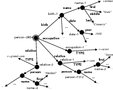
 relative person name first
 .
.
Data-classes. Any equivalence class over the nodes of the graph qualifies as a data-class. Data-classes are similar to semantic tags in other contexts. I will describe now the data-classes I use in my work, but other definitions are possible (for example, path plus frame types across the path), a subject I am interested in pursuing in further work (Chapter 9, Section 9.2).
Data-paths.
As domain independent
data-classes,2
I employed paths in the knowledge representation (data-paths). I need to identify particular
pieces of knowledge inside the graph. I thus select a particular frame as the root
of the graph (the person whose biography I am generating, in my case —doubly
circled in the figure) and consider the paths in the graph as identifiers for the different
pieces of data. Each path will identify a class of values, given the fact that some
attributes are list-valued (e.g., the relative attribute in the figure). I use the notation
 to denote these data paths (Figure 3.1 shows an
example).
to denote these data paths (Figure 3.1 shows an
example).
Text. A text is a sequence of words.
Concept.
To compute statistics over knowledge representations, I need a means to decompose
them into statistical events. A concept is anything that can be asserted to be true or false (false
as a negation of true) given a knowledge representation. To avoid data sparseness I employ
concepts in the form of a data-path to an atomic node and the value of the atomic node (e.g.,
 ). More complex concepts can include decision logic (e.g.,
value > 35) and mix several atomic nodes, a subject I started some preliminary investigations
(Duboue, 2004). To clarify, based on this definition,
). More complex concepts can include decision logic (e.g.,
value > 35) and mix several atomic nodes, a subject I started some preliminary investigations
(Duboue, 2004). To clarify, based on this definition,  and
and
 are different concepts.
  is a data-path (a
type of data-class), and not a concept.
is a data-path (a
type of data-class), and not a concept.
Phrase. In the same vein, phrases provide a way to decompose a text into statistical events over which statistics can be computed. In my work, I have used uni-grams as phrases (bi-grams in preliminary investigations (Duboue and McKeown, 2003a)). This decision was also taken to avoid data sparseness. In general, patterns over the text (e.g., “found x out”) would make for ideal phrases.
Verbalization Dictionary. A function that takes a concept as input and returns a set of phrases that can potentially verbalize the given concept.
Matched Text. A matched text (an example is shown in Figure 3.2) is a text where selected phrases are linked to concepts.3 The data-path provide a semantic tag for the piece of matched text.
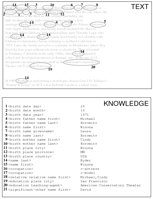
 ) in the knowledge representation.
My work can be termed Indirect Supervised Learning4 because my training material is fully supervised but the input/output pairs do not have the information needed for direct learning. I thus have input (the knowledge representation), output (text) and a hidden class (the document plans). I want to learn the mapping from input to the hidden class (how to build document plans from a knowledge source, the task of the strategic component in a NLG system) and I have a model of the mapping from the hidden class to the output (from document plans to texts, the remainder of the NLG system). The key is that I want to learn the estimator for the hidden class together with the estimator for the text to the hidden class. While I could have a classifier that assigns sets of observed outputs to values of the hidden class, I am actually trying to approximate this classifier from some independence assumptions.5
My current model assumes that the hidden class (the document plan) is the only element needed to determine the wording in the text (an independence assumption). I thus consider the text to be randomly sampled from all the texts that verbalize the document plan (Figure 3.3). Therefore, Indirect Supervised Learning has two steps; in the first step, the indirect training material (natural dataset) is transformed into direct training material (the hidden class is elucidated). In the second step, output learning representations are learned in a supervised way, from the training dataset constructed in the previous step.
A different alternative I explore in Chapter 6 is to compute the output of the hidden class, that is, to produce text from the document plans and then use text-to-text metrics for learning. However, as I am not learning the transformation from document plans to final text, the verbalization becomes a deterministic step where no parameters are estimated, and will therefore be a source of constant noise.6

The evaluation process I follow for my Indirect Supervised Learning task is also a contribution of this thesis, as it lets me evaluate both the supervised and unsupervised steps at the same time. Given the training material, I divide it into train (Tr) and test (Te) sets. I then proceed to hand-annotate the test set (Te).
To evaluate the unsupervised part, I join Tr +Te (again, only to evaluate the unsupervised part) and induce annotations automatically (by virtue of the unsupervised nature of the process) over the whole Tr+Te set. Now, I bring back the human annotations over Te and use them to evaluate the quality of the automatically assigned annotations. This measures the quality of the training material for the supervised part.
To evaluate the supervised system, I execute the unsupervised system again, but now only over Tr alone. I then use the annotations automatically obtained over Tr to train the supervised system and execute it over Te (that was not available during training at any point) and compare it to the quality of the human annotations over Te. This measures the generalization power of the technique.
I evaluate the matched texts extrinsically for Content Selection and Document Structuring. The extrinsic evaluation (how good are the matched texts with respect to selection and ordering) is motivated by the fact that I do not have a gold standard matched text constructed by hand; instead, I have annotated the selection labels on the text set and ordered them by first mention on the text.
As a Content Selection metric, I use precision (P ), recall (R) and F* measure, from information retrieval (van Rijsbergen, 1979). They are defined as:
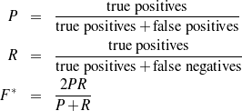
Where true positives is the number of atoms present in both the hand-tagged test set and the automatically constructed matched texts. The number of items wrongly included becomes the number of false positives. Finally, the items that should have been included but were missed are the number of false negatives.
To evaluate statistical significance of the results, I followed (Mitchell, 1997), pages 146-147, and divide Tr and Te into three non-overlapping folds. In each fold, I executed different variants of the system and then compare their differences in error rate on each fold. This constitutes a case of a paired experiment (every system is trained and tested in the same data). Because each of the sets is non-overlapping, this setting makes for more reliable statistics. For each fold, the error rate E defined as
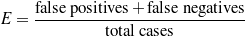
is computed. Then the error differences δi in each fold are computed. Therefore, given three
folds (Tr1,Te1), (Tr2,Te2), (Tr3,Te3) and two system variants  A, B, each variant is trained
in (Tr1 +Te1), (Tr2 +Te2), (Tr3 +Te3) and tested in Te1,Te2,Te3. Then defining:
A, B, each variant is trained
in (Tr1 +Te1), (Tr2 +Te2), (Tr3 +Te3) and tested in Te1,Te2,Te3. Then defining:
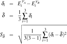
The true difference in the two variants lies in the interval

Where is the mean of the differences and S is an estimator for the standard deviation of the differences. The t2,N are the t-values for two degrees of freedom and they depend on the confidence interval (N%). They are given by the following table:
| N = | 90% | 95% | 98% | 99% |
| t = | 2.92 | 4.30 | 6.96 | 9.92 |
As a Document Structuring metric, I employ Kendall’s τ correlation coefficient (Lebanon and Lafferty, 2002) between the elements common to the hand-tagged test set and the automatically obtained training material:
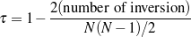
Where N is the number of atomic values in the intersection and inversions is the number of exchanges on consecutive objects required to put them in the order appearing in the hand tagged reference. This metric ranges over the interval [-1.0,1.0] with a value of 1.0 meaning perfect correlation, 0.0 no correlation and -1.0 inverse correlation. As explained in Chapter 5, this is an accepted metric for ordering in text structure (Lapata, 2003).
In this section, I detail how general training material, in the form of Text and Knowledge is transformed into a matched text, a training material that can be used for both the task of learning Content Selection rules and Document Structuring schemata.
Indirect supervised learning involves an unsupervised step, based on assumptions on the
structure of the model, to elucidate the hidden variable and supervised steps to generalize from
the constructed mapping. My assumptions are related to the ways knowledge can appear on
the text. This model is summarized by the following two tests, where H0 is the null
hypothesis, p and c are particular phrases and concepts, is the set of phrases that
make a particular text, is the set of concepts that make a particular knowledge
representation (where and refer to the same entity) and is the verbalization
dictionary:
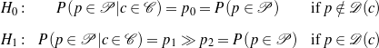
The null hypothesis H0 (an independence equation) can be paraphrased as
saying that if a phrase p does not belong to the verbalization dictionary for a given
concept c, then, for a given text (decomposed into a set of phrases ), knowing
that the concept belongs to the knowledge representation associated with that
text7
does not affect the chances of the phrase p appearing in the text. On the contrary, H1 says that
the chances are much greater if the phrase p does belong to the verbalization dictionary of c.
This model is inspired by the work of (Dunning, 1993). It is clear that, given a verbalization
dictionary , the matched text construction reduces to a disambiguation task. My experiments,
however, use H0 and H1 in an attempt to elucidate the while constructing the matched
texts.
In a sense, I am using the existence of a concept in a particular knowledge representation
as a way to partition the set of all knowledge representations. For example, I can use the
concept of being a comedian  to put together all the data of
comedians vs. non-comedians. I then want to see if I can observe changes on the distribution
of phrases over the texts associated with the partitions. This statistical test selects
words that are then added to the verbalization dictionary (Figure 3.4). I will now
analyze each of the components of the system (Concept Enumeration and Statistical
Filtering).8
to put together all the data of
comedians vs. non-comedians. I then want to see if I can observe changes on the distribution
of phrases over the texts associated with the partitions. This statistical test selects
words that are then added to the verbalization dictionary (Figure 3.4). I will now
analyze each of the components of the system (Concept Enumeration and Statistical
Filtering).8
The dictionary induction starts by enumerating all possible concepts that can be asserted over a
set of knowledge representations. This process starts by enumerating all paths in a composite
graph (e.g.,  ) and then checking the possible values that can be
found at the end of each path for each of the input knowledge representations (e.g.,
) and then checking the possible values that can be
found at the end of each path for each of the input knowledge representations (e.g.,
 for Winona Ryder,
 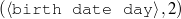 for Pablo Duboue
and so on). Concepts found this way make for a large total number (the concept enumeration
can generate as many as 20,000 concepts in a given run). Only concepts that are true for a
minimum number of knowledge representations (the concept’s support) are used. More
complex concepts can be enumerated via clustering (Duboue and McKeown, 2003b).
Thus open class sets are only enumerated for their more common elements (e.g.,
first-name=“John”). In my experiments, I use a support value of thrsupp, as shown in
Table 3.10.
for Pablo Duboue
and so on). Concepts found this way make for a large total number (the concept enumeration
can generate as many as 20,000 concepts in a given run). Only concepts that are true for a
minimum number of knowledge representations (the concept’s support) are used. More
complex concepts can be enumerated via clustering (Duboue and McKeown, 2003b).
Thus open class sets are only enumerated for their more common elements (e.g.,
first-name=“John”). In my experiments, I use a support value of thrsupp, as shown in
Table 3.10.
I then compare the distribution of phrases in the partition of texts associated with the partition in the knowledge representations induced by the concept.9 That is to say, I want to see if there is a change in the distribution of words between the two sets; for example, if the biographies of people born in ‘MI’ (a concept) have a higher-than-expected chance of containing the phrase “Michigan.”
Therefore, I have two sets of texts (Michigan and non-Michigan) and I analyze if they diverge in their associated language models over phrases; if they represent samples coming from two different distributions. To achieve this goal, I collect phrasal counts (uni-grams over words in my case) and analyze whether or not these counts can be considered samples coming from the same probability distribution. I collect counts over all phrases (i.e., words in my case). This process is schematically represented by the pseudo-code shown in Figure 3.5.
C ←∅ ; set of all concepts
P ←∅ ; set of all phrases
ForEach (T,K) ∈ set of all text-knowledge pairs Do
C ← C∪ set of all concepts in K
P ← P ∪ set of all phrases in T
Done
ForEach concept c ∈ C Do
s ←∅ ; all text-knowledge pairs where c holds
ns ←∅ ; all text-knowledge pairs where c does not hold
ForEach (T,K) ∈ set of all text-knowledge pairs Do
If c holds on K Then
s ← s∪{(T,K)}
Else
ns ← s∪{(T,K)}
Fi
Done
; look for words associated with the partition s/ns
ForEach p ∈ P Do
Countss=Array[100]
Countsns=Array[100]
ForEach i = 1..100 Do
Samples=select at random 5 texts from s
Samplens=select at random 5 texts from ns
Countss[i]=number of times p appears in Samples
Countsns[i]=number of times p appears in Samplens
Done
If Countss and Countsns are stat. sig. different Then
Add p to the verbalization dictionary for c
Fi
Done
Done
Student’s t-test. I investigated statistical tests on the counts for each phrase on either partition. In my statistical test, I test the null hypothesis that these words appeared there just by chance. For example, if the partition is induced by the concept “his or her occupation is to be a comedian,” I want to conclude that their associated biographies contain the phrases (i.e., words) “comedian,” “stand-up,” and “comic” more than expected by chance on this corpus.
There might be other terms found frequently for a given concept that are not exact verbalizations of that concept. For example, for people born in Michigan, phrases like “Upper Peninsula” or “Detroit” are to be expected. Therefore, this approach might over-generate.
I compared three statistical tests χ2, likelihood ratios and Student’s t-test. My counts were too small for χ2, likelihood ratios do not allow for the sampling process described below and therefore only Student’s t-test is used as part of the final algorithm.
I have the total number of occurrences of the events (in this case, phrases) and I want to see if a phrase is associated with the partition induced by the concept. Therefore, as shown in the pseudo-code in Figure 3.8, I split the texts into two sets, the texts belonging to the partition, and the texts that do not belong to the partition. If I apply likelihood ratios or similar techniques to the counts associated with the whole clusters, usually the most descriptive phrases for each element in the cluster will prevail (e.g., in the case of biographies, the names of the people involved in the cluster will appear).10 I thus resort to a sampling process to avoid this effect. I sample sets of five texts from the partition and five from texts outside and collect phrasal counts. After several samples (100 in my case), I end up with two sequences of numbers, representing the number of times a given phrase appear in each partition; to determine if the two sequences of numbers belong to the same distribution I use the Student’s t-test.11 If the test results are over a threshold thrt (see Table 3.10), I consider the phrase to be a verbalization adding it to the verbalization dictionary.
The output of the dictionary induction process is a verbalization dictionary containing sets of putative verbalizations for each concept. An example of newly added words is shown in Figure 3.6. I only evaluated this dictionary extrinsically, my measuring its impact on the quality of the obtained matched texts.


The verbalize-and-search process (Figure 3.7) aims to identify pieces from the input that
contain known verbalizations in the target text. It enriches a matched text initialized with plain
target texts. The verbalization step takes a concept and returns all the phrases associated with
the concept in the verbalization dictionary.
For example, given a concept such as ( , “John”), I will search for the
strings “John”,“J.” and “JOHN”. To search for the phrases in the text, any classical
search algorithm can be employed, e.g., KMP or Boyer-Moore (Gusfield, 1997).
, “John”), I will search for the
strings “John”,“J.” and “JOHN”. To search for the phrases in the text, any classical
search algorithm can be employed, e.g., KMP or Boyer-Moore (Gusfield, 1997).
The overall operation is prone to two type of errors: omission (if the verbalization dictionary misses the exact verbalization, e.g., c-comedian appears in the text as “he performed comedy for several years” or “MA” instead of “Maryland”) and over-generation (if there are several values for it, e.g., “Smith” appears in the text and it is simultaneously the name of the father and a brother). The former errors were addressed by the dictionary induction technique described in the previous section. The latter errors are addressed by means of disambiguation methods explained below.
The ambiguity problem in the verbalize-and-search approach cannot be overlooked. For
example, Winona Ryder was born in a city named Winona, in Minnesota. When the phrase
“Winona” is found in the text whether the previous words are “born in” or “born as” can
provide strong indication for either usage. To acquire the contexts (“born in” vs. “born as”)
for each data-class ( vs.
vs.  ), I compute all ambiguous
matches across documents and use standard disambiguation techniques (Naïve Bayes) to
smooth12
the evidence and decide for each class against a null model (trained in every word in the
document). This is a local disambiguation, using a very small window (w = 3, see
Table 3.10).
), I compute all ambiguous
matches across documents and use standard disambiguation techniques (Naïve Bayes) to
smooth12
the evidence and decide for each class against a null model (trained in every word in the
document). This is a local disambiguation, using a very small window (w = 3, see
Table 3.10).
In other words, I accumulate statistics for matching at the data-class level. Each match is delimited by a context and all the contexts are accumulated across all the members of the class. This process works on the assumption that, for example, the words surrounding the name of a relative are the same across names of relatives and different biographies. Therefore, I have my list of verbalizations and the places where they match, some of these matches are spurious matches, but working on the hypothesis that the good matches still outnumber the spurious ones (something that is normally the case), I collect statistics from all these contexts. Figure 3.8 shows pseudo-code for this process.
NullModel←∅
ForEach T ∈ all available texts Do
ForEach word in place w ∈ T Do
Train NullModel for a small context (window = 3) around w
Done
Done
M ←∅ ; all matches
ForEach (T,K) ∈ set of all text-knowledge pairs Do
ForEach concept c ∈ K Do
M ← M∪ set of all matches in T for a verbalization of c
Done
Done
PathModeldata-paths ←∅
ForEach data-path d ∈ all possible data-paths Do
ForEach match m ∈ M such that path of m equals to d Do
Train PathModeld for a small context (window = 3) around m
Done
Done
MatchesToAdd←∅
ForEach match m ∈ M Do
If PathModel path of m (m) > NullModel(m) Then
Add m to MatchesToAdd ordered by the score of PathModel
Fi
Done
Moreover, I retrain the disambiguators after some matches have been identified to
improve their generalization capabilities. For example, if my system has successfully
identified an occurrence of “Ryder” in the text “Winona Ryder is an actress” as
 , it can use it later to disambiguate “Winona” as
  rather than
 .
.
While my final system uses Naïve Bayes disambiguation, I also investigated three other variants, shown in Table 3.1 (this experiment was done on the biography.com corpus mentioned later in this chapter). In the table, the strict variants refer to whether to require that only the left or right context decides in favor of the class (regular variant) or to require that both contexts decide in favor of the class (strict variant). My experiments with the strict variant did not confirm the intuition that it should provide a higher precision, therefore I discontinued its use. I also re-implemented a HMM-based disambiguator following the IdentiFinder trainable named-entity system (Bikel et al., 1999). My implementation, however, did not include the complex class-based smoothing complexities described by Bikel et al., with an inferior performance to the Naïve Bayes approach. I thus decided to focus on the Naïve Bayes technique.
| Disambiguation Method | Precision | Recall | F-measure
|
| Naïve Bayes | 0.706± 0.007 | 0.681± 0.013 | 0.694± 0.010 |
| Naïve Bayes (Strict) | 0.636± 0.028 | 0.416± 0.007 | 0.503± 0.013 |
| HMM | 0.698± 0.016 | 0.543± 0.009 | 0.611± 0.006 |
| HMM (Strict) | 0.526± 0.011 | 0.057± 0.015 | 0.100± 0.022 |
The Text-Knowledge corpus used in this chapter consists of knowledge extracted from a semi-structured knowledge base, biographical fact-sheets of assorted celebrities. These fact-sheets were crawled from E! on-line13 in November 2002. In addition to this knowledge source, I also employ an extended knowledge source, also extracted from E! on-line but with a slightly different ontology and with added information about which movies each actor appeared in. This extended knowledge source was incorporated as part of these experiments at the end of this dissertation and was not used during system development (i.e., no parameters were fit on this corpus). Different biographical sites provide the text part, to test the ability of the system to learn from different types of data. The process of constructing this Text-Knowledge corpus is detailed in Chapter 7, Section 7.1, I will just detail here the overall size of each Text-Knowledge corpus. As explained in Section 3.2.1, each corpus was split into a training and test set, with the test set tagged for selection and ordering (ordering only in the last corpus) by the author.
The biography.com corpus is the smallest (in number of pairs) corpus of the collection and it was used mostly for development. The biographies are clearly written by professional editors and present the higher level of homogeneity.
| biography.com | Total | Average | Train | Test
|
| # pairs | 102 | - | 91 | 11 |
| # frames | 4,956 | 45.588 | 4,442 | 514 |
| # triples | 10,628 | 104.196 | 9,500 | 1,128 |
| # words | 54,001 | 529.422 ± 301.15 | 49,220 | 4,781 |
| # chars | 337,775 | 3,311.520 ± 1,857.96 | 307,978 | 29,797 |
In the table, pairs refer to the number of text and knowledge pairs; frames refer to the number of internal nodes in the graph; triples refer to the number of triples in the form (frame, link, target), the equivalent of an arrow in Figure 3.1; words and chars refer to the number of words and characters in the target texts, respectively. The average number of words per biography and its standard deviation speaks of quite lengthy biographies with a stable length (compared to the next two corpora).
The test set contains 334 selected triples, from a total of 744 triples to select from (an F*14 for the Select-All strategy of 0.62 —The Select-All strategy can be thought of as a baseline). The total number of triples is different than the number shown in the table as the table also shows triples that connect internal nodes.
This corpus was a fine development corpus, as its small size allowed me to implement and test different ideas quite quickly. On the other hand, this corpus constitutes a high baseline that makes it difficult to appreciate the relative differences of system variants. For that reason, I introduced the other corpora detailed next, each of which presents a relatively harder matched text construction task.
The s9.com corpus is the largest corpus (in number of pairs) and the one with the shortest biographies. The biographies are mostly one-liners and it is unclear whether or not they have been written by editorial staff.
| s9.com | Total | Average | Train | Test
|
| # pairs | 578 | - | 558 | 20 |
| # frames | 30,709 | 53.130 | 29,723 | 986 |
| # triples | 95,032 | 164.415 | 92,969 | 2,063 |
| # words | 21,037 | 36.396 ± 34.04 | 20,192 | 845 |
| # chars | 138,711 | 239.984 ± 215.82 | 133,204 | 5,507 |
Because of the small size of each biography, this is a challenging corpus, where out of 1,377 triples to select from, only 170 are selected (an F* for the Select-All strategy of 0.22). The texts are so small (36 words on average) that one would be hard pressed to call them biographies. The standard deviation is also pretty large.
In previous work (Duboue and McKeown, 2003a, Duboue, 2004), I have used the corpus assembled from imdb.com as a test corpus. It is of medium size and has biographies submitted by volunteers over the Web; this made it more challenging than corpora written by an editorial staff.
| imdb.com | Total | Average | Train | Test
|
| # pairs | 199 | - | 185 | 14 |
| # frames | 10,123 | 50.869 | 9,362 | 761 |
| # triples | 31,676 | 159.176 | 29,323 | 2,353 |
| # words | 64,196 | 322.593 ± 285.63 | 60,086 | 4,110 |
| # chars | 378,778 | 1,903.407 ± 1,693.88 | 354,560 | 24,218 |
The test set contains a total of 369 selected triples out of 1,060 (an F* for Select-All of 0.516). While the size of each biography is around 300 words, so is the standard deviation; and thus, the biographies on this corpus are clearly of diverging sizes.
Near the end of this dissertation work, I created an extended knowledge source by adding to the previous knowledge extra information in the form of artistic credits (the movie starred by each actor). This extended knowledge source was paired against biographies from wikipedia.org. The site wikipedia.org is a collaborative collection of encyclopedic articles embodied in the concept of a Wiki, a page that allows any person with WWW access to edit it. The Wiki approach produces a very dynamic set of pages that pose a more challenging environment than the previous corpora. On the bright side, this corpus contains more pairs than the imdb.com and it has a very liberal license that allows for corpus re-distribution. This is the only corpus annotated with ordering information, because the extended knowledge source is the only one compatible with the hand-written communicative predicates presented in Chapter 5. These predicates are a requirement for learning Document Structuring schemata.
| wikipedia.org | Total | Average | Train | Test
|
| # pairs | 361 | - | 341 | 20 |
| # frames | 58,387 | 161.737 | 55,326 | 3,061 |
| # triples | 108,009 | 299.194 | 102,297 | 5,712 |
| # words | 68,953 | 191.006 ± 55.17 | 64,784 | 4,169 |
| # chars | 418,035 | 1,157.992 ± 334.01 | 392,925 | 25,110 |
The test set contains 598 selected triples out of 2,906 (an F* for Select-All of 0.341).
The architecture presented in the previous sections leaves room for a number of variations, some of which I have investigated in this thesis. I investigated the following issues:
Addition of the matches to the matched text being constructed. As mentioned in Section 3.3.2, it is advantageous to retrain the disambiguators after a certain number of matches have been identified. I investigated two possibilities for adding matches to the partial matched text. I describe them below.
Creation of the verbalization dictionary. While in this thesis I focus on the automatic construction of the verbalization dictionary (Section 3.3.1), this dictionary can be obtained in a number of ways, some of which do not necessarily include learning:
 , the verbalization is John. This will obviously not
work in the case the value is not phrase, e.g.,
, the verbalization is John. This will obviously not
work in the case the value is not phrase, e.g.,  .
.
I explored these options through the following variants:
The results for the Content Selection quality of the learned matched texts are shown in Table 3.2.
Variant 1 was computationally too expensive to compute on the larger corpora and only biography.com results are included. The relative differences between Variant 1 and Variant 2 can only be seen if we plot precision and recall during the matched text construction process (Figure 3.9 and Figure 3.10). The figures are obtained by evaluating the matched text being constructed as matches are being added to the matched text. The y-axis measures precision and recall and the x-axis are iterations on the matched text construction process. These figures show clearly how Variant 1 starts very well until its curves suddenly drop (around the tenth iteration), most likely because it commits itself to add all matched instances in a wrongly matched data-path. Variant 2, on the other hand, has a much softer curve, where the benefits of re-training the disambiguators on earlier matches can be seen clearly;15 even precision improves after some matches have been identified.
In general, Variant 0 has the best precision across all corpora, with Variant 4 presenting the best recall. When considering F*-measure, Variant 4 has the best F* overall, although that is not the case in all corpora.
Because of the differences in Table 3.2 are pretty small, I conducted a cross-fold validation experiment to test the differences between the variants. The actual results of these experiments are presented in Appendix A. I will mention here the highlights. For biography.com, only Variant 1 has a statistically significant difference with a good level of confidence. For s9.com and imdb.com, no difference has a good confidence, although the difference between variants 3 and 4 in imdb.com is noteworthy. In wikipedia.org, the differences between Variant 2 and the Variants 0 and Variants 3 are statistically significant with good confidence.
In this evaluation, the system is trained in (Tr+Te) and tested in Te (as explained in Section 3.2.1). Here Tr is used to provide extra evidence to the dictionary induction and disambiguation methods. This approach begs the question of the importance of the size of Tr for the results reported over Te. Moreover, because the cross-validation experiments that measure statistical significance are trained in one third of Tr each fold, it is also important to understand how different such system may be with respect to the system trained in all Tr. Figure 3.11 and Figure 3.12 show the impact of the size of Tr for Variants 2 and 3 in 10 different random subsets of different size (10,11,..,30, 40, ..., 90) of Tr (plus all Te) and testing the obtained labels on Te. The figures show clearly that Variant 2 requires at least 60 instances to stabilize, while Variant 3 (that does not performs any dictionary induction) profits from the extra training material very slowly (by improving the disambiguators).
Variant 0 (Pathadd+ Trivialdict)
| Corpus | Prec. | Rec. | F* | selected |
| biography.com | 0.7407 | 0.6432 | 0.6885 | 297 |
| s9.com | 0.5108 | 0.5280 | 0.5193 | 184 |
| imdb.com | 0.7118 | 0.5303 | 0.6078 | 295 |
| wikipedia.org | 0.6952 | 0.4664 | 0.5583 | 420 |
Variant 1 (Pathadd+ On-linedict)
| Corpus | Prec. | Rec. | F* | selected |
| biography.com | 0.7112 | 0.6842 | 0.6974 | 329 |
Variant 2 (Scoreadd+ Off-linedict)
| Corpus | Prec. | Rec. | F* | selected |
| biography.com | 0.7508 | 0.6676 | 0.7068 | 297 |
| s9.com | 0.5000 | 0.5529 | 0.5251 | 188 |
| imdb.com | 0.7035 | 0.5338 | 0.6070 | 280 |
| wikipedia.org | 0.6190 | 0.4782 | 0.5396 | 462 |
Variant 3 (Scoreadd+ Externaldict)
| Corpus | Prec. | Rec. | F* | selected |
| biography.com | 0.7335 | 0.6347 | 0.6805 | 289 |
| s9.com | 0.5026 | 0.5529 | 0.5266 | 187 |
| imdb.com | 0.6853 | 0.5311 | 0.5984 | 286 |
| wikipedia.org | 0.6280 | 0.5083 | 0.5619 | 484 |
Variant 4 (Scoreadd+ Externaldict+ Off-linedict)
| Corpus | Prec. | Rec. | F* | selected |
| biography.com | 0.7466 | 0.6706 | 0.7066 | 300 |
| s9.com | 0.5193 | 0.5529 | 0.5356 | 181 |
| imdb.com | 0.6830 | 0.5941 | 0.5941 | 284 |
| wikipedia.org | 0.6451 | 0.5183 | 0.5746 | 481 |
Finally, to shed further light on the differences in Table 3.2, I analyzed the error over
each data-path. Tables 3.3 and 3.4 show major contributors to the error and success rates,
respectively. These contributors perform similarly across all variants. There we can see that the
free-text paths (for example, paths that end in canned-text in this particular knowledge
representation) and the symbolic paths (paths that finish in #TYPE, for example) are responsible
for a large number of errors. On the other end of the spectrum (more successful paths), there are
paths such as  or
or 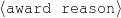 (movie names and the like) that have
higher chances of appearing in the text exactly as they appear in the knowledge representation
(they are stronger anchors, in the nomenclature of Chapter 1). These are data-paths
containing more named-entity alike information and they are better captured by my
system.
(movie names and the like) that have
higher chances of appearing in the text exactly as they appear in the knowledge representation
(they are stronger anchors, in the nomenclature of Chapter 1). These are data-paths
containing more named-entity alike information and they are better captured by my
system.
While my system has no provisions for free-text values, the dictionary induction should
deal with the #TYPE paths. This can be seen in Tables 3.5-3.8 that show error
contribution itemized per variant for data-paths with variant-related differences. In
biography.com corpus, for example the table shows that the variants with dictionary
induction (Variants 1 and 2) mildly address the symbolic fields with Variant 1 marginally
better than Variant 2. This is to be expected as Variant 1 does a very costly on-line
dictionary induction, where the dictionary is re-induced after some matches are identified
(improving the quality of the language models). With respect to the differences coming
from the use of disambiguation, this can be appreciated in the last name of relatives
( ). However, the use of disambiguators makes the whole
system more wary of places where little evidence across frames supports the match (the system
becomes more conservative). This situation slightly increases the number of mismatches in a
number of paths.
). However, the use of disambiguators makes the whole
system more wary of places where little evidence across frames supports the match (the system
becomes more conservative). This situation slightly increases the number of mismatches in a
number of paths.
The error analysis for the s9.com corpus (Table 3.6) shows the same overall behavior of biography.com, although here the disambiguation improves more paths than in biography.com. Interestingly, as the system becomes more conservative, the gains equalize again. This is because I am averaging over all paths. The table shows how the distribution of errors is more uniform thanks to the disambiguated system. This will be particularly important for the ordering behavior in the wikipedia.org corpus.
Table 3.7 contains the misses per data-path in imdb.com, which are also in line with
the previous two corpora. Note how  benefits from the small
external dictionary in Variant 3.
benefits from the small
external dictionary in Variant 3.
biography.com
| s9.com
|
||||||||||||||||||
imdb.com
| wikipedia.org
|
biography.com
| s9.com
|
|||||||||||||||||||||||||||
imdb.com
| wikipedia.org
|
| path | misses per variant | total
| |||
0 | 1 | 2 | 3 | to select | |
| claimtofame canned-text | 11 | 10 | 11 | 11 | 11 |
| occupation #TYPE | 16 | 10 | 13 | 16 | 16 |
| significant-other #TYPE | 15 | 14 | 15 | 15 | 15 |
| relative #TYPE | 17 | 16 | 15 | 17 | 17 |
| relative relative name last | 9 | 6 | 5 | 5 | 11 |
| education teaching-agent name | 3 | 3 | 4 | 4 | 7 |
| significant-other significant-other name first | 1 | 1 | 2 | 2 | 15 |
| significant-other significant-other name last | 1 | 1 | 2 | 3 | 13 |
| award subtitle | 4 | 5 | 4 | 4 | 11 |
| award date year | 3 | 3 | 6 | 6 | 21 |
| relative relative name first | 1 | 1 | 3 | 5 | 14 |
| path | variant | total
| ||
0 | 2 | 3 | to select | |
| birth father name last | 2 | 1 | 1 | 2 |
| birth name last | 11 | 8 | 7 | 13 |
| birth name first | 5 | 5 | 3 | 14 |
| name first | 0 | 1 | 3 | 16 |
| relative relative name last | 3 | 2 | 3 | 5 |
| path | variant | total
| ||
0 | 2 | 3 | to select | |
| birth father name last | 5 | 0 | 1 | 5 |
| education place country | 1 | 0 | 0 | 1 |
| birth place province | 6 | 6 | 0 | 8 |
| relative relative name last | 11 | 2 | 4 | 12 |
| name first | 0 | 5 | 5 | 14 |
| name last | 0 | 9 | 9 | 14 |
| significant-other significant-other name first | 0 | 0 | 2 | 9 |
| award date year | 2 | 5 | 5 | 13 |
| path | variant | total
| ||
0 | 2 | 3 | to select | |
| birth name last-name | 6 | 2 | 3 | 6 |
| birth place province | 10 | 10 | 1 | 10 |
| birth date-instant month | 19 | 16 | 1 | 19 |
| #TYPE | 20 | 15 | 20 | 20 |
| education place province | 1 | 1 | 0 | 3 |
| name last-name | 0 | 2 | 4 | 20 |
| name first-name | 0 | 1 | 1 | 20 |
| work-event reason name name | 3 | 3 | 4 | 16 |
| family relative name last-name | 13 | 5 | 4 | 18 |
| significant-other significant-other name last-name | 2 | 2 | 3 | 18 |
| significant-other significant-other name first-name | 1 | 3 | 2 | 17 |
| family relative name first-name | 0 | 1 | 1 | 26 |
| work-event date-instant year | 11 | 12 | 12 | 51 |
| work-event built name name | 20 | 24 | 21 | 66 |
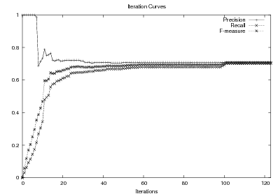
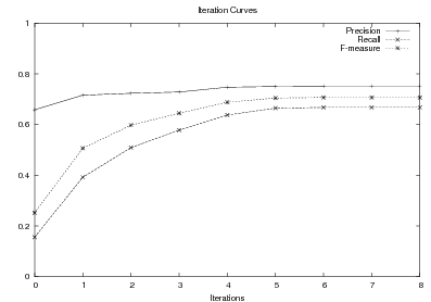
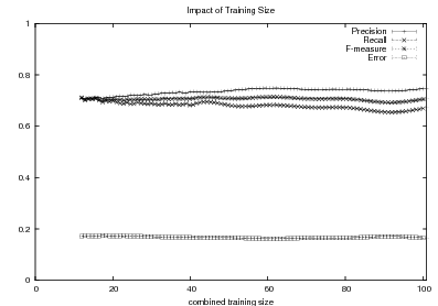
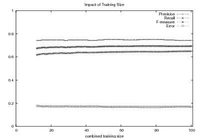
The results for Document Structuring on the wikipedia.org corpus are shown in Table 3.9. While the sequences are similar in length to the text set, according to Table 3.2 only half of the information there appears also in the test set. For these elements in the intersection, there is a near-perfect correlation in the ordering. This implies this data can be used positively to learn Document Structuring schemata.
The sequences evaluated here are sequences of atomic values as they appear in the matched text. These sequences are different from sequences of instantiated communicative predicates (such sequences are document plans) but they will nevertheless be used in Chapter 5 to evaluate different schemata during learning. The sequences of atomic values will also be used to learn Order Constraints.
Variant | avg. length | τ
| ||
| 0 | (Pathadd+ Trivialdict) | 21.55 ± 7.7083 | 0.9400 ± 0.0989 | |
| 2 | (Scoreadd+ Off-linedict) | 23.10 ± 8.3470 | 0.8686 ± 0.1283 | |
| 3 | (Scoreadd+ Externaldict) | 26.50 ± 12.2280 | 0.9232 ± 0.1004 | |
| 4 | (Scoreadd+ Externaldict+ Off-linedict) | 26.35 ± 11.4260 | 0.8909 ± 0.1154 | |
The process presented in this chapter is able to automatically identify training material with an F*-measure as high as 0.70 and as low as 0.53 and a τ as high as 0.94 and as low as 0.86. These results imply that learning using the matched texts as training material will require a robust machine learning methodology as the ones introduced in the next two chapters.
Moreover, as it will be discussed in Chapter 8, the technique presented here cannot learn after a certain point. Particularly, it has problems with free-text fields (e.g., “claim to fame”) or facts included in the text out of being of extraordinary nature.
| Threshold | Description | Value |
| thrt | t-test cut-point | 9.9 |
| thradd | Percentage of the available number of matches to run
the on-line dictionary induction. | 20% |
| thrtop | Number of top scoring matches to add in each step
(computed as a percentage of the total number of
matches). | 10% |
| w | Disambiguation window, in words. | 3 |
| thrsupp | Concept support, in percentage of the total number of
instances. | 20% |
This chapter presents my work on the automatic acquisition of a set of Content Selection rules. These rules provide a particular solution to the Content Selection task (a task defined in the next section). I decided to use these symbolic rules (also described in the next section) as a representation for learning because they capture the requirements of my Content Selection problem. Moreover, they are also easy to understand by humans, allowing the output of the learning system to be further refined for quality, if needed.
The internals of this rule learning process are the focus of this chapter. The rule learning mechanism described here learns from the ideal dataset for the task of learning Content Selection rules: knowledge data with select (sel) or omit (¬sel) labels (Figure 4.1 (b)). Such training material can be considered ideal for learning Content Selection logic as it is the input and output of the Content Selection process. The labels will thus signal, for each piece of data, whether or not the piece of data should be selected for inclusion in the final text. The ideal dataset can be obtained directly by hand-tagging but I am interested in a solution without any human intervention, neither from a knowledge engineer or annotators. Therefore, I learn from a noisy approximation obtained from the natural dataset for the task, in the form of a Text-Knowledge corpus (Figure 4.1 (a)), using the matched text from the previous chapter.1 The Supervised Learning step (Section 4.2) will thus search for rules that better accommodate this training material. The training material from the biographies domain sketched in the previous chapter (Section 3.4, discussed at length in Chapter 7, Section 7.1) will be used to run a number of experiments, presented in Section 4.3.
Learning from a dataset extracted automatically makes for a very challenging task. For instance, my approach of analyzing how variations in the data affect the text (used to build the matched texts in the previous chapter) is prone to over-generation, as explained in the limitations chapter, Section 8.2. This over-generation implies that the rules learned from this dataset will be likely to have low precision.
|
|
||||||||||||||||||
| ⇓ | ⇓ | ||||||||||||||||||
| Sean
Connery, born Thomas
Sean Connery in August
25th, 1930 in Scotland
is an actor, director and
producer. … |
|
||||||||||||||||||
| (a) | (b) | ||||||||||||||||||
| label | data-path | value |
| sel |  | “Sean” |
| sel |  | “Connery” |
| ¬sel |  | 84Kg |
| ¬sel |  | 188cm |
| sel |  | “Oscar” |
| ¬sel |  | “MTV” |
| sel |  | c-grand-son |
| sel |  | “Dashiel” |
| ¬sel |  | c-step-cousin |
| ¬sel |  | “Jason” |
I will now introduce some definitions I use in the remainder of this chapter.
Content Selection. This is the action of choosing the right information to communicate in a NLG system, a complex and domain dependent task. Figure 4.2 shows an example; its input is a set of attribute-value pairs, and its output is a subset of the input attribute-value pairs, determined by the selection labels (sel or ¬sel). The labeled with sel subset contains the information that will make up the final, generated text. Content Selection can be thought of as a filtering or as a labelling process. When thought of as a labelling process, the system will choose between two labels: sel (i.e., filter accepts) or ¬sel (i.e., filter rejects). The labelling approach allows for a generalized Content Selection task, where each piece of data is assigned a salience score. In my work, I will consider a labelling task with two classes. My approach can be extended to accommodate generic classes as discussed in the Conclusions chapter (Section 9.2).
Content Selection rules.
The output of my learning system are Content Selection rules, which base their decision
solely on the available knowledge. All rules are functions from a node to  ; that is, they
take a node in the knowledge representation and return true or false. In this way, my Content
Selection rules contain decision logic only for atomic nodes. In this chapter, expressions such
as “a piece of data to be selected” are formalized as an atomic node in the knowledge
representation graph (of all types but Reference type, see the definitions in the previous
chapter). The decision of whether to include a given piece of data is made solely on the given
data (no text is available during generation, as the generation process is creating output text).
Sometimes it is enough only to analyze the value of the atomic node (e.g., to tell an Oscar
from a BAFTA award). In other cases, however, it is also necessary to look at the
surrounding information to decide whether or not to include a piece of data. For
example, to tell the name of a cousin from the name of a grand-son (Figure 4.3) or to
tell a successful movie (movies that received a number of awards) from failures. A
simplifying assumption involved in a two level Content Selection approach, as the
one presented in this thesis, is that all nodes are processed independently during
the first Content Selection level. Therefore, the outcome of the decision about other
nodes is not part of a given node decision. This simplifying assumption is clearly
wrong (in a extreme case, if a piece of information appears repeated as two different
nodes, the inclusion of one node should prevent the other node to be included), but
Content Selection in context is attacked by the fitness function presented in the next
chapter.
; that is, they
take a node in the knowledge representation and return true or false. In this way, my Content
Selection rules contain decision logic only for atomic nodes. In this chapter, expressions such
as “a piece of data to be selected” are formalized as an atomic node in the knowledge
representation graph (of all types but Reference type, see the definitions in the previous
chapter). The decision of whether to include a given piece of data is made solely on the given
data (no text is available during generation, as the generation process is creating output text).
Sometimes it is enough only to analyze the value of the atomic node (e.g., to tell an Oscar
from a BAFTA award). In other cases, however, it is also necessary to look at the
surrounding information to decide whether or not to include a piece of data. For
example, to tell the name of a cousin from the name of a grand-son (Figure 4.3) or to
tell a successful movie (movies that received a number of awards) from failures. A
simplifying assumption involved in a two level Content Selection approach, as the
one presented in this thesis, is that all nodes are processed independently during
the first Content Selection level. Therefore, the outcome of the decision about other
nodes is not part of a given node decision. This simplifying assumption is clearly
wrong (in a extreme case, if a piece of information appears repeated as two different
nodes, the inclusion of one node should prevent the other node to be included), but
Content Selection in context is attacked by the fitness function presented in the next
chapter.
I mine a different set of rules for each data-class (data-path in my case). The impact of the data-class equivalence classes for the quality of Content Selection rules is a subject I am interested in pursuing in further work.
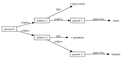
 .
.
Select-All/Select-None rules.
The first type of rules, Select-All/Select-None, addresses the first four rows of
Figure 4.2. After analyzing a number of target biographies in a hypothetical style, it is easy to
see that the first and last names of the person being described should always be included in the
biography. Conversely, his weight or height should never be included. These rules will
select or omit each and every instance of a given data-class at the same time (e.g., if
 is selected, then “Dashiel” and “Jason” will both be selected in
Figure 4.2).2
is selected, then “Dashiel” and “Jason” will both be selected in
Figure 4.2).2
Tri-partite rules. After careful analysis of my training data and experimentation with different rule languages, I have settled for rules containing three pieces of information (these rules are applied to an atomic node in the graph, the ‘current node’):
The constraints can be very general (including access to global variables or arithmetic
operations on Numeric nodes), but in my work I have used two simple constraints. The first
constraint, True, always selects the information for inclusion. It is marked as ‘-’ in my
representation of the rules. The second type of constraints are constraints saying that the value
of the node has to belong to a set of values. They are marked as ‘value ∈ ’. The tri-partite
rules can contain empty paths (denoted as ‘-’), in which case there should be no constraints on
the second node.
’. The tri-partite
rules can contain empty paths (denoted as ‘-’), in which case there should be no constraints on
the second node.
This rule language addresses three types of selection needs, all shown in the example knowledge base with selection labels of Figure 4.2. To begin with, it is possible to express Select-All/Select-None rules in this language (first two rules in Figure 4.4), successfully addressing the first four rows of Figure 4.2.
The next two rows, regarding different awards the person has received make for a more interesting case, where the information should be included only if it belongs to a certain set of important values. In the celebrities domain, important awards include, for example, Oscars or the Golden Globes (motivating rules such as the third one in Figure 4.4). Obviously, the relative importance of the different awards is clearly domain dependent. The case shown in the figure is paradigmatic: MTV movie awards are seldom mentioned in target biographies. This omission is to be expected according to people I consulted who are interested in celebrities issues. Nothing a priori in the data prepare you for that result, as MTV is a source of authority in the celebrities domain. As the experiments in Section 4.3 show, my system is able to acquire this type of information.
Finally, for the last four rows in Figure 4.2, the information to solve the selection of the name of the relative does not lie on the name itself but in the value of another node that can be reached from the name node: the type of the relation. This fact motivates the path and the constraints in the other node (as part of the tri-partite rule). My final goal has been to be able to express with the rules concepts as complex as this movie should be selected if it received an Oscar, as shown in the last rule of Figure 4.4.
 (-, -, -). ;Select-All
Always say the first name of the person being described.
 : (false, -, -). ;Select-None
Never say the eye color of the person being described.
 : (value ∈
 , -,-).
Only mention the name of an award if it is whether a Golden Globe or an Oscar.
 : (-,
: (-, ,value ∈
 ).
).
Only mention the title of a movie if the movie received an Oscar.
Complex Content Selection Rules. In preliminary investigations (Duboue, 2004), I presented a variant of my system that targets more complex rules than the tri-partite ones I have just defined. These rules allow for recursion and are summarized in Figure 4.5. While this rules are more expressive than the tri-partite ones, I discontinue their use in favor of the tri-partite rules, as the latter are a more constrained representation that makes better use of the training material.
 , that
is, they take a node in the knowledge representation and return true or false. These rules
are more expressive than their simplified counterpart.
, that
is, they take a node in the knowledge representation and return true or false. These rules
are more expressive than their simplified counterpart.
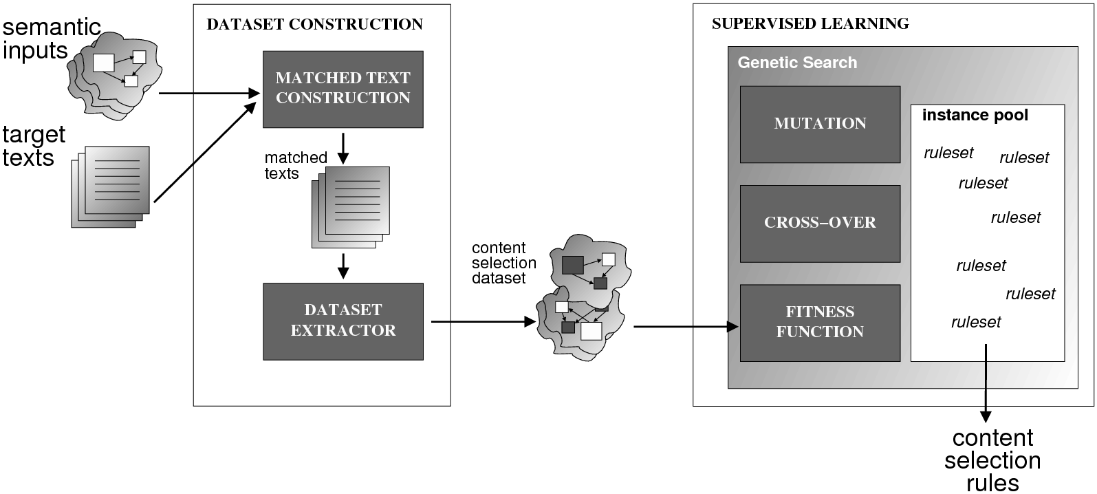
Figure 4.6 illustrates my two-step indirect supervised learning approach, divided into a number of modules. The first step, Dataset Construction (discussed in the previous chapter), turns the aligned Text-Knowledge corpus into a training dataset consisting of knowledge and selected or omitted labels (the Relevant Knowledge). Once the labels have been elucidated, the Supervised Learning module performs a Genetic Search in the space of possible rulesets, as described in this section.
I have thus a dataset consisting of classification labels (selected, sel, or omitted, ¬sel) for each piece of input knowledge. I want to learn that mapping (from concept to classification label) and capture that information about the mapping using Content Selection rules. This constitutes a case for Supervised Learning. The information available to the learner is thus the frame knowledge representation (a graph) plus the labels. This implies learning from structural information (as compared to learning from flat feature vectors). To this end, several alternatives are possible, including using memory-based learning, inductive logic programming, combinatorial algorithms and kernel methods (Washio and Motoda, 2003). Given the high dimensionality of the decision space over graphs, I have found it valuable to be able to define a successor instance coming from two instances in the search pool, instead of one. This type of approach is known as Genetic Algorithms (Section 4.2.1). In general, I consider GAs as a meaningful way to perform symbolic learning with statistical methods. To motivate its use I also propose a comparison to ML classification systems in Section 4.2.2 and to some meaningful baselines in Section 4.2.3.
 | ||||||||||||||||
| ↓ | ||||||||||||||||
| rule | ||||||||||||||||
|
||||||||||||||||
| ↓ | training | |||||||||||||||
 | ← F-measure → |  |
||||||||||||||
I have input and output pairs of knowledge and labels (K,L), with labels extracted from the matched text. I am interested in finding the rules r* (belonging to the set of all possible Content Selection rules) such that r* maximizes the posterior probability given the training material:
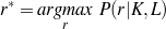
instead of computing a probability, I use the input and output pairs to compute for each putative rules r a likelihood f(r,K,L) that allows me to compare among them. This likelihood is thus a quality function in the representation space. I use the rules (r) to generate from the input knowledge K a set of labels L′. The sought quality function becomes the distance between the training output and the produced output, ||L-L′||. As distance, I use the F-measure from Information Retrieval (IR). This process is sketched in Figure 4.7.
With the quality function in hand, finding the rules r* implies a search process on the large space of representations. The key ingredients in a Genetic Algorithms solution are the fitness function (the quality function mentioned above), the operators and the initial population. I will describe them shortly.
Fitness Function. The fitness function takes a tri-partite rule r and computes its expected goodness with respect to the training material. One contribution of this thesis is to employ as fitness function the Fα measure (weighted f-measure from IR (van Rijsbergen, 1979)) of the classification task of recovering all selection labels on the training datasets. That is to say, for a given data-class, there are a number of items in the data-class to be selected according to the training material. The tri-partite rule r is applied to the knowledge and the number of correctly selected items becomes the rule’s number of true positives. The number of items the rule wrongly selects is its number of false positives. Finally, the items the rule should have selected but it missed are the rule’s number of false negatives. The Fα then is defined as follows, where P stands for precision and R stands for recall:
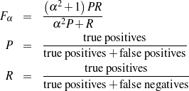
The fitness function is the key to learning using GAs. In earlier versions of my system the fitness function was too biased towards selecting all elements in the data-class. The key ingredient for a successful function in my problem has been to add information about the priors for each class (selected or omitted) in each data-class. The function defined above implicitly incorporate these priors (in the counts of false positives and false negatives).
As I wanted to obtain rules with higher recall than precision, I employed α = 2.0 (recall is doubly as important as precision), as shown in Table 4.5. I added a minimum description length (MDL) term to the fitness function to avoid over-fitting the data (by memorizing all training instances). The final fitness function is then:

MDL term.
To avoid overtraining I use a MDL term as part of the fitness function. The type of
over-training I try to avoid are, for example, cases where month-of-birth is always
selected but I only see all months but June in the training material. There a rule like
(value ∈ “Sep”,
  , -,-)
will accomodate the training material, but (-,-,-) (True) will also explain it, and generalize
better.
, -,-)
will accomodate the training material, but (-,-,-) (True) will also explain it, and generalize
better.
Coming up with this MDL term was much harder that I expected as easy choices were either too strong and dominated the fitness function or were too weak and failed to avoid over-training completely. I defined the final MDL function as:
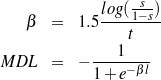
Where t is the total number of items to be selected in the current data class, s is a user-provided saturation parameter (I used 0.99 in my experiments, see Table 4.5) and l is the length of the rule being evaluated measured in characters.
This MDL term is a heuristic function with the following justification: it is a negative value between 0 and -1.0. When combined with the Fα (that ranges between 0 and 1.0), the resulting fitness function will range between -1.0 and 1.0. The MDL function is a sigmoid with two saturation regions controlled by the s parameter. In one saturation region, the function will evaluate to 0 (no MDL penalty) and in the other it will evaluate to -1.0 (MDL rejects completely). Outside the saturation area, the function is quasi-linear, with its slope depending on the number of selected items to be selected (data classes with more items to be selected tolerate more complex rules).
The use of MDL to increase generalization capabilities is inspired by the tree pruning performed in C4.5 (Quinlan, 1993). The sigmoid function is similar to sigmoid activation functions for neural networks (Hertz et al., 1991).
|
|
|
↕ |
↕ |
|
|
|
↓ |
↓ |
c |
|
c |
I have a cross-over operator (Figure 4.8) that takes the two rules and combines them into a new one, by following these steps: first, the constraints in the node are merged, when merging constraints, there is a 50% chance that the constraints are copied from only one parent (a parent decided proportionally to its fitness value). The other 50% chance goes to 25% chance of picking the union of the constraints and a 25% chance of picking the intersection of the constraints (although an empty intersection is promoted to True). Then it looks at whether the two parents share the same path (the second entry in the tri-partite rule) or not. If they share the same path, the constraints in the second node are merged. Otherwise, one parent is selected (again, fitness-proportional), and its path and constraints copied to the child.
While cross-over takes two instances to create the new instance, mutation operations work on an existing instance, producing a new instance with a variation of the original. I investigated three possible variations, detailed below: growing the existing instance, shrinking the existing instance, and shuffling the existing instance.
The grow mutation will, with equal probability, add a new random value to check for in the constraints for the node and the node at the end of the path. The shrink mutation will remove a value from the constraints (if there is any value to remove). Finally, the shuffle mutation will change the path in the rule with a new path taken randomly from the set of all possible paths. The constraint at the end of the path will also be selected randomly.
Initial Population. I do not use the genetic algorithm to explore different paths; it only explores the space of constraints over nodes. The paths are exhaustively enumerated when building the initial population, until a maximum distance from the node (breath-first search, depth in Table 4.5) is reached. To obtain these paths, a composite graph is created from all training instances. Moreover, the selection and distribution of atomic values at each node in the composite graph is also recorded. This distribution is used to create initial constraints for the paths obtained via breath-first search. Other areas of the graph do not contribute to the construction of the initial population.
Stopping Criteria. I considered two stopping criteria for the genetic search. The first one was an overall maximum number of generations. The second criteria has to do with lack of changes in the overall population. When the best instance found so far stays the same for a certain number of generations, the population is considered to have converged to a maximum.
I use Weka (Witten and Frank, 2000), a framework containing a number of supervised automatic classification algorithms, to provide an alternative solution to the Content Selection task. Weka machine learning algorithms take as input a fixed-size feature-vectors with fixed types representing the relevant information for each instance, together with its target class, in my case select or omit.
My traditional ML module takes the full data for a person, together with the selected labels and transforms this information into training material for the Weka classification system. I trained binary classifiers (selected or omitted) for each data-path. The main problem resolved in this module is how to represent a graph-based knowledge representation using flat feature vectors. My solution to this problem is explained below.
Given the highly structured frame knowledge representation (a DAG, with values in the leaves and attributes in the connecting links), to obtain a flat structure it was necessary to create a structure that encompasses all the possible input structures, and later linearize it. I employed the following algorithm to propositionalize my input graphs: first, I turned the graph into exactly one tree, by taking a spanning tree rooted in the node4 to be selected or omitted, with maximum depth (normally between 3 to 6). Each of these trees could be traversed to obtain a flat vector. However, I needed to be able to represent all possible (available) trees in a simple vector. In that vector, a fixed coordinate has to have the same meaning across trees. For example, in the celebrities domain each tree represents one person, so I wanted coordinate 89 for Marilyn Monroe to be “name of the third cousin” and coordinate 89 for Warren Beaty to be also “name of the third cousin.” As different inputs may have defined different attributes (for example, in the medical domain a patient may have a key tachycardia-start-time while other may have bradycardia-start-time), and some attributes may be duplicated several times (for example, the patient may have had several drugs administered during the surgery, all of them are values for the drugs-given attribute), I needed a means to record and fix the possible attributes appearing at every node, together with the possible number of values (“fan-out”) each of these attributes can take (in the case of multiple-valued keys, like award or relative). For this purpose, I build a unifier tree for all the training trees. The process of building such a tree is summarized in Figure 4.9.
This unifier is built from training examples. Given enough of them, I expect to be able to capture all the possible attributes seen in an arbitrary input with its corresponding fan-outs. In the worst case, there will be data in an input that the Weka classifier will not be able to use for classification, providing suboptimal, but possibly adequate, results.
With such a unifier, a flat attribute-vector representation can be obtained by simultaneously traversing both the unifier and the tree at hand, producing default values in the case of non-existent data in the target tree or the occurring value otherwise. Finally, the module automatically assigns types to each coordinate of the output vector. I identify three types: numerical values, strings belonging to a small subset of possible values (Weka nominal type, such a “mg”, “mcg” and “g” for units of measurement) and strings from an open set that receive only one boolean entry representing whether it is defined or not.
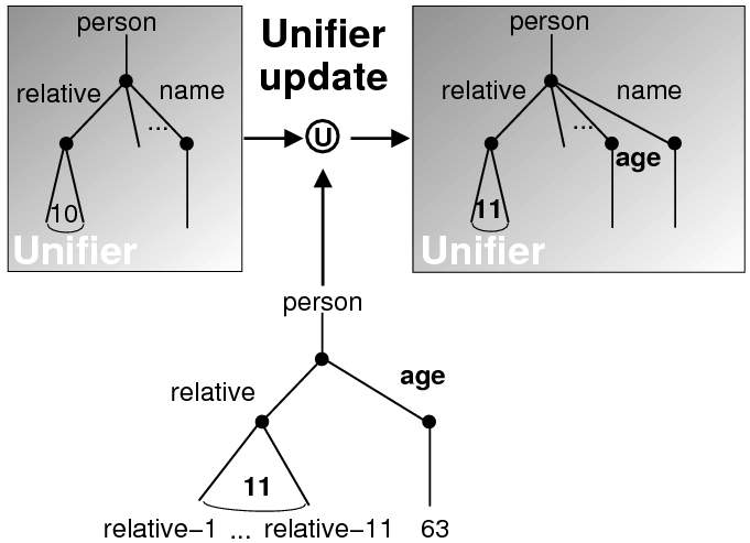
This propositionalization process generated a large number of features, e.g., if one person had a grandmother, then there will be a “grandmother” column for every person. This situation gets more complicated when list-valued values are taken into consideration. In the biographies domain, an average-sized 100-triples biography spanned over 500 entries in the feature vector, even after pruning it for entries that are invariant in the training data.
The training vectors can be generated by the procedure described above for both the automatically obtained datasets and the hand-tagged evaluation set. After training on in the automatically obtained training material (one classifier per data-path), the combined system is tested on the unseen test vectors.
In Section 4.3, I compared the following machine learning techniques:
Recent additions to Weka allow for set-valued features, in the form of the jRip package (re-implementing the RIPPER algorithm (Cohen, 1996)). Such additions would allow to use parts of paths as features, but they were not available at the time of these experiments.
As baseline, I use Select-All/Select-None rules over the baseline matched text described in the last chapter, Section 3.5 (matched texts without dictionary induction nor disambiguation). This solution involves counting how many items in each data-path appear as selected in the training material and then choosing the strategy Select-All or Select-None if the F* for the path is greater than 0.5 (I use the F* as a way to equally balance precision and recall). This algorithm maximizes the overall F* for the path-based Select-All/Select-None strategy. When mined from matched texts obtained through the Variant 0 system in the previous chapter (Section 3.5), they provide a meaningful baseline for comparison. When mined from Variant 4 matched texts (Duboue and McKeown, 2003a), they provide a simpler alternative to the rules presented in this chapter, as they are faster to execute and less prone to errors coming from the assemblage of the matched text. Select-All/Select-None rules, however, still require a good level of post-filtering in later stages (they over-generate quite a bit) and may miss relevant information.
To shed further light on the relative strengths of the methods described in this chapter, I ran a number of experiments. First, I learned Select-All/Select-None rules (Table 4.1). I learned the rules from the Variant 0 matched texts (Section 3.5) to obtain some baseline rules. I also learned from Variant 4 matched texts (matched texts with a combination of dictionary induction and external verbalization dictionary). The table shows that, while the differences in intrinsic quality reported in the previous chapter for the two variants was small (less than two percentual points in the F*), it translates in a major difference in the type of Select-All/Select-None rules that can be learned from them (an extrinsic evaluation). Moreover, Select-All/Select-None rules mined on Variant 4 are a good competitor to tri-partite rules, as presented next.
| Variant 0 | Variant 4 | |||||||
| Corpus | P | R | F* | sel | P | R | F* | sel
|
| biography.com | 0.6023 | 0.6077 | 0.6050 | 36 | 0.5785 | 0.6616 | 0.6173 | 55 |
| s9.com | 0.3542 | 0.4647 | 0.4020 | 11 | 0.5000 | 0.4823 | 0.4910 | 18 |
| imdb.com | 0.5841 | 0.3197 | 0.4133 | 22 | 0.5269 | 0.3712 | 0.4356 | 39 |
| wikipedia.org | 0.8515 | 0.1822 | 0.3002 | 10 | 0.5884 | 0.2892 | 0.3878 | 33 |
Using again the best available matched texts (Variant 4), I learned tri-partite rules per Section 4.2.1 (Figure 4.10 illustrates some of the rules learned). The results over the four corpora are shown in Table 4.2. These results improve several points over the baseline, while all but s9.com improve over Variant 4 rules. The improvement is more marked in some corpora than others. For example, the improvements over biography.com are moderate but note that the rules are six points from the F* of the training material The wikipedia.org corpus presents the higher improvement over the baseline (13 points in F*-measure). That illustrates how my learning system can profit from a larger knowledge pool. The fact that Select-All/Select-None rules on Variant 4 for the s9.com corpus perform better than the tri-partite rules over the same corpus supports the hypothesis that Select-All/Select-None rules are to be preferred in the presence of high noise.
Appendix A shows that Variant 4 has a high confidence statistically significant difference with the baseline for all corpora but imdb.com. In wikipedia.org, the rules also present good confidence for the difference between Select-All/Select-None rules and the baseline.
 (-, -, -) True;
  (-, -, -) True
 (value ∈
 , -, -)
As I used U.S. biographies, the country of education is only mentioned when
it is abroad.
 (value ∈
 , -, -)
Mention sisters and step-fathers.
 (value ∈
 , -, -)
Mention husband and wives (but not necessarily boyfriends, girlfriends or
lovers).
| Corpus | P | R | F* | sel |
| biography.com | 0.5829 | 0.7155 | 0.6424 | 410 |
| s9.com | 0.3387 | 0.4941 | 0.4019 | 248 |
| imdb.com | 0.5029 | 0.4607 | 0.4809 | 338 |
| wikipedia.org | 0.5150 | 0.3729 | 0.4325 | 433 |
Using the biography.com Variant 4 training material, traditional ML classification systems were trained and tested, following Section 4.2.2. The results are shown in Table 4.3. Because all the results are below baseline (0.60 in Table 4.1), it may be the case that the unification/spanning-tree approach described in Section 4.2.2 is generating too many features for the small training material available. This hypothesis is supported by the fact that logistic regression is the approach that fares better in Table 4.3.
| Metric | j48 (C4.5) | Naïve Bayes | SMO (SVM) | Logistic
|
| Precision | 0.6790 | 0.6226 | 0.6086 | 0.6161 |
| Recall | 0.4940 | 0.4940 | 0.5029 | 0.5718 |
| F* | 0.5719 | 0.5509 | 0.5508 | 0.5931 |
To further validate my tri-partite rule induction system, I ran the system under different values of the α parameter (Figure 4.11). The figure attests that the α parameter works as expected, producing rules with a stable F* but varying degrees of precision and recall controlled by the α parameter. The importance of these results cannot be overlooked, as they show how my approach can be tuned to learn broad rules or highly precise rules, from an automatically obtained training material.
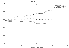
Finally, I tested whether the rules being learned were different or not by running them across corpora. Table 4.4 shows a 3×3 grid obtained by training the system in each of the three corpora and testing it in each of the three corpora (wikipedia.org is in a different knowledge representation so it could not be used). The figure clearly illustrates how the rules learned are different for each corpus. Interestingly, the rules learned on biography.com perform better in s9.com than the rules learned on s9.com themselves. The matched texts for s9.com are so noisy that quality rules for the domain learned in a higher quality corpus perform better than rules learning in a very noisy approximation to the corpus itself. This result encourages work not now in generating a particular biography style, but selecting data that adheres to a biographical domain. That is, given information about a person, certain information would be more naturally fit to be included into a biography (it can be selected on the basis of the biographical domain). Categorizing information in this way is different from the task targeted in this thesis, where a particular style of biographies was sought to be mimicked. The domain-related task results in a summarization problem. Adapting my technique to summarization is an issue I am interested in addressing in future work (Chapter 9, Section 9.2).
| Tested | Trained on | |||||
| on | biography.com | s9.com | imdb.com
| |||
| biography.com | 0.58290.7155 | 0.6424 | 0.16830.7941 | 0.2777 | 0.40130.6666 | 0.5010 |
| s9.com | 0.65920.3532 | 0.4600 | 0.33870.4941 | 0.4019 | 0.46230.2493 | 0.3239 |
| imdb.com | 0.55650.3682 | 0.4432 | 0.22950.5941 | 0.3311 | 0.50290.4607 | 0.4809 |
The technique targeting learning Content Selection rules presented in this chapter is able to effectively learn rules from the noisy matched texts. Moreover, it is noticeable how the differences between the different matched text variants get a boost when used to learn Content Selection rules.
An alternative approach using traditional machine learning methods suffers from a data sparsity problem that speaks in favor of techniques specifically designed to target the Content Selection problem.
While the rules mined in this chapter are ready to be used in a generation system, as mentioned in the conclusions of the previous chapter, it is necessary to model free-text fields (e.g., “claim to fame”) or facts included in the text out of being of extraordinary nature to make progress beyond the results presented here.
| Threshold | Description | Value |
| populationsize | Size of the population in the genetic search for
Content Selection rules. | 1000 |
| depth | Depth cut-off for the breath-first search building the
population for the rule search. | 6 |
| α | F-measure weighting. | 2.0 |
| l | Saturation area of the MDL sigmoid function. | 0.99 |
This chapter describes my learning technique to acquire Document Structuring schemata from an aligned Text-Knowledge corpus. As mentioned in Chapter 3, my learning has two steps: an unsupervised step and a supervised step. The unsupervised step in this case involves building the matched texts (per Chapter 3, Section 3.3); and then mining sequences of atomic values and order constraints (presented here, Section 5.2). For the supervised process of learning Document Structuring schemata (Section 5.4), I use a fitness function based on three items: Content Selection, order constraints and sequence alignment.
This technique is evaluated in two domains: Medical Reports (next chapter), where it enjoyed limited success and Biographical Descriptions (Chapter 7) where some of the problems encountered point to needed improvements discussed in Chapter 8.
I will now introduce some key concepts used in the rest of this chapter.
For learning Document Structuring schemata, I use as input the aligned Text-Knowledge corpus and a set of communicative predicates. The Text-Knowledge corpus has already been introduced in Chapter 3. I will define here the communicative predicates. Moreover, one of the contributions of this dissertation is OpenSchema (Duboue, 2005), a declarative definition of the Document Structuring schemata, also presented in this section. These schemata are compatible with (McKeown, 1985)’s original definition, discussed in chapter 2, Section 2.2.1.
Document Structuring Task. The Document Structuring task takes as input a subset of the knowledge base (the relevant knowledge pool) and returns a sequence of messages (a document plan). These messages are produced by the predicates defined below.
Communicative Predicates. Each predicate (Figure 5.1) is composed of three items: variables, properties and output. Each variable has a type, which further constrains the possible values it can take (an item of that type or subtype, given an ontology). These variables range over frame references. Following KNIGHT, MAGIC and similar systems, I use domain dependent predicates (instead of (McKeown, 1985) rhetorical predicates). I call these predicates communicative predicates, as they hold a good deal of Domain Communication Knowledge, DCK (Chapter 2, Section 2.2). The actual number and nature of these predicates varies from domain to domain. In my implementation these predicates are defined in a constraint satisfaction formalism. For the discussion that follows, a predicate can be considered as a function that takes a number of defined (and maybe undefined) variables and searches the knowledge representation for values of the undefined variables that satisfy the constraints inside the predicate. If none are found (or if the provided variables do not satisfy the constraints), the predicate cannot be instantiated. For each set of values1 that satisfy its constraints, the predicate produces a message (Figure 5.2), a data structure assembled using the variable assignment found during the search. The messages are the nexus between the schema and the rest of the NLG system. A predicate, therefore, can be thought of in this context as a blueprint for making messages. In this thesis, I use functional descriptions (FDs) as messages, as I work with a FUF/SURGE (Elhadad and Robin, 1996) based implementation. The details of the messages are important because I will later need a means to compare these messages (the output of the schema) to sequences of atomic values (that I can read out from matched texts).
Document Plan. A document plan is a sequence of messages produced by predicates instantiated from variables ranging over frames in the knowledge representation.
| person | : | c-person |
| education-event | : | c-education-event |

My Declarative Schemata. Given a set of predicates, a schema (Figure 5.3) is a finite state machine over the language of predicates with variable references. All the variables in the schema are global variables, to distinguish them from the predicate variables (local variables). At each step during schema instantiation, a current node is kept and all the predicates in the edges departing from the current node are instantiated (via the process sketched in the previous definition). A focus mechanism (coming directly from (McKeown, 1985) and thus described in Chapter 2, Section 2.2.1) will then select the next node (and add the message to the document plan), situations with 12 or more possible continuations during schema instantiation have been found in practice. The instantiation process finishes when no new predicate can be instantiated departing from the current node. While the schema itself is simple (an automaton with predicate and variable names on its edges), the instantiation process is complex because it has to keep track of free (i.e., undefined) and bound variables (predicates bind variables;2 some variables can also be bound before the instantiation begins —as global arguments of the schema, for example, the person being described in the biography) and focus stacks. Interestingly, my schema induction algorithm makes no assumptions on the instantiation process, being therefore independent of the instantiation process or its internal details (e.g., the local search strategy —focus in my case). This makes for a very knowledge lean approach with a wider range of application. However, this complex instantiation process forbids using existing learning techniques for finite state machines (FSMs) to learn the schemata. This situation arises as a finite state machine will produce all the strings belonging to its language. A schema contains a FSM but will produce a much smaller set of strings, only the ones licensed by the FSM and the focus mechanism. This situation cannot be overlooked: if we believe that schemata explain the data we are observing (the human data), then the only strings being observed are the ones valid according to the focus mechanism. Therefore, there will not be enough data to elucidate the original FSM by using only FSM-learning techniques.


 *
* 
 *
*
Other-Work-Event(person↔self)*


∥

 *
*

 *
*

To learn Document Structuring schemata, I have matched texts and a set of predicates. As mentioned in the previous section, a schemata takes relevant knowledge as input and produces as output document plans. Examples of these document plans would be needed to supervisedly learn schemata. The document plans, however, are not readable from the matched texts, as they contain no mention of the rhetorical predicates. For example, assume there are two predicates: occupation and date-of-birth. Both take two arguments, occupation takes a person and an occupation and date-of-birth takes a person and a date-of-birth. Then, for the text
“John Doe is an actor. John Doe was born on 1/1/80.”
generated from the sequence of two instantiated predicates:
occupation(person-1, occupation-1/type) date-of-birth(person-1, date-1/month, date-1/day, date-1/year).
the matched text will only contain the eight-item sequence of atomic values:
name-1/first name-1/last occupation-1/type name-1/first name-1/last date-1/month date-1/day date-1/year
but no reference to the predicates occupation and date-of-birth.
Moreover, the matched text construction process has no provisions for anaphoric expressions. As a result, only the first mention will be reliably identified. Therefore, if the above example is laid out more naturally as
“John Doe is an actor. He was born on 1/1/80.”
The sequence of atomic values will thus be reduced to
name-1/first name-1/last occupation-1/type date-1/month date-1/day date-1/year
My system does not resolve “He” to “John Doe,” so it misses the second mention. That is to say, the matched text can reliably provide the placement information for the first mention of the atomic value in question (in general, first mentions are always easier to identify (Jansche, 2003)). The sequences mentioned below, extracted from the matched text will thus be cleaned for repeated values after the first mention (to ensure compatible results in cases where second mention were not identified).
To learn the schemata I then focus on three items that can be extracted from the matched texts:
These three elements will be used to implement a fitness function in the schemata space. This function (described in Section 5.4.2) will not utilize the semantic sequences directly, but will profit from order constraints mined over such sequences. These order constraints are also useful to produce a baseline to compare against the learned schemata. They are the focus of the next section.
name-24→first-name name-24→last-name date-24→year date-24→month date-24→day name-30→first-name award-1→title name-40→first-name sister-relative-1→Type date-7→year date-30→year date-2→year date-26→year date-36→year date-27→year date-34→year date-35→year date-14→year date-23→year date-16→year date-1→year date-12→year wn-musician-2-1→Type name-18→name |                         |
|
| (a) | (b) | |
This section describes the mining and usage of order constraints over the placement of semantic types over text (data-paths as used in this thesis, data-classes in the general case). These sequences can be read directly from the text (after it has been matched against the knowledge representation as in Chapter 3 or it has been hand annotated as will be presented in the next chapter). As such, they can be mined from annotated texts, as described in the next section.
The order constraints can be then used to measure how felicitous a given document plan is. For that, a semantic sequence can be read out from the document plan. Because the predicates contain no ordering information over the atomic values used to instantiate them, a technique for approximate matching over sequences of sets (each set representing an instantiated predicate) is discussed in Section 5.3.2.
As mentioned in the previous section, to learn the order constraints, I extract from the matched text the sequence of data-classes (data-paths), a sequence that I call a semantic sequence (in Figure 5.4, from the sequence of atomic values (a), the semantic sequence is (b)). I base my unsupervised learning algorithm on techniques used in computational genomics (Durbin et al., 1998), where patterns representing meaningful biological features are discovered from large amounts of seemingly unorganized genetic sequences. In my application, I search for patterns that occur repeatedly across multiple semantic sequences. By learning ordering constraints over these elements, I produce constraints that allow later selection of the schema that better explains the training material. My system uses combinatorial pattern matching (Rigoutsos and Floratos, 1998) combined with clustering to learn patterns. Subsequently, it applies statistical procedures to learn ordering constraints among these clusters of patterns.
The algorithm can be sketched as follows: I applied combinatorial pattern discovery (detailed in the next section) to the semantic sequences. The obtained patterns are refined through clustering. Counting procedures are then used to estimate order constraints between the clusters.
Pattern Detection. Pattern discovery techniques are often used for information extraction (e.g., (Riloff, 1993, Fisher et al., 1995)), but most work uses data that contains patterns labelled with the semantic slot the pattern fills. Given the difficulty for humans in finding patterns systematically in my data, I needed unsupervised techniques such as those developed in computational genomics, where patterns of the type I need are called motifs.
As explained by (Hudak and McClure, 1999), motif detection is usually addressed with alignment techniques (as mentioned by (Durbin et al., 1998)) or with combinatorial pattern discovery techniques such as the ones I use here. Combinatorial pattern discovery is more appropriate for my task because it allows for matching across patterns with permutations, for representation of wild cards and for use on smaller data sets.
I will now provide a brief explanation of my pattern discovery methodology. The explanation builds on the definitions below:
 pattern.
  *Σ, where ? represents a don’t care (wild-card) position. The
 parameters are used to further control the amount and placement of the
don’t cares: in every subsequence of length W, at least L positions must be filled
(i.e., they are non-wild-cards characters). This definition entails that L ≤ W and
also that a
parameters are used to further control the amount and placement of the
don’t cares: in every subsequence of length W, at least L positions must be filled
(i.e., they are non-wild-cards characters). This definition entails that L ≤ W and
also that a  pattern is also a
  pattern, etc.
Using the previous definitions, the algorithm reduces to the problem of, given a set of
sequences, integers L and W , a minimum window size, and a support threshold, finding
maximal  -patterns with at least a support of support threshold. My implementation can
be sketched as follows:
-patterns with at least a support of support threshold. My implementation can
be sketched as follows:
 patterns with support greater than support threshold (described in
Table 5.1 are kept. Figure 5.7 shows an example.
patterns with support greater than support threshold (described in
Table 5.1 are kept. Figure 5.7 shows an example.
Clustering. After the detection of patterns is finished, the number of patterns is relatively large. Moreover, as they have fixed length, they tend to be pretty similar. In fact, many tend to have their support from the same subsequences in the corpus. As I was interested in similarity in form as well as similarity in context, a convenient solution was to further cluster the patterns, according to an approximate matching distance measure among patterns.
An approximate matching measure is defined for a given extended pattern. The extended pattern is represented as a sequence of sets; defined positions have a singleton set, while wild-card positions contain the non-zero probability elements in their don’t care model. Consider p to be such a pattern, S a sequence and o an offset over S, the approximate matching is defined by
![∑length(p)match (p[i],S[i+ o])
^m(p,o,S ) = -i=0-----------------------
length(p)](thesis176x.png)
where the match(P,e) function is defined as 0 if e ∈ P , 1 otherwise, and where P is the set at position i in the extended pattern p and e is an element of the sequence S. This measure falls in the interval [0,1]. Using this function, I defined the approximate matching distance measure (one way) between a pattern p1 and a pattern p2 as the sum (averaged over the length of the offset list of p1) of all the approximate matching measures of p2 over the offset list of p1. This is, again, a real number in [0,1]. To ensure symmetry, I defined the distance between p1 and p2 as the average between the one way distance between p1 and p2 and between p2 and p1.
This metric provides an approximate measure of how well a given pattern does match in the contexts where other pattern matches, if the original pattern is “forced” to match there. If two patterns are fully compatible, this metric will give a score of 1.0. If they are completely incompatible, it will give a score of 0.0.
I used agglomerative clustering with the distance between clusters defined as the maximum pairwise distance between elements of the two clusters. Clustering stops when no inter-cluster distance falls below a user-defined threshold. An example is shown in Figure 5.8.
intraop-problems intraop-problems 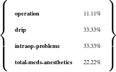
drip
intraop-problems 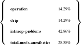
drip drip
intraop-problems intraop-problems 
drip drip
Constraints Inference. The last step of my algorithm measures the frequencies of all possible order constraints among pairs of clusters and atomic values, retaining those that occur often enough to be considered important, according to a relevancy measure. The algorithm proceeds as follows: a table counting how many times a pair of patterns belonging to particular clusters or atomic values are matched and appear in a particular order is built. From there, I use (Shaw and Hatzivassiloglou, 1999) approach (discussed in the Related Work chapter, Section 2.3, repeated here for clarity).
In the table of counts, therefore, the entry at position i,j indicates the number of times in the corpus the object i came before the object j. From the table, I can try to reject the null hypothesis that i,j came in any order (equivalent to say that the probability of i coming before j is 0.5). The following formula will compute the probability of the observed frequencies:

where m is the total number of times i has been seen occurring before j in the corpus and n is total number of times i and j occur in a pair. I thus use the above equation with a threshold throc (Table 5.1) to select “likely enough” constraints.
I will describe in this section how order constraints can be used to evaluate a schema being constructed or as a stand-alone planning mechanism, but first I will explain how to evaluate the constraints themselves.
I evaluated two items: how effective4 the patterns and constraints learned were in an unseen test set and how accurate5 will report the number of patterns, clusters and constraints learned during training. These figures are the upper bound for the number of patterns, clusters and constraints found on unseen, held-out sequences. The number of constraints found is particularly important as only constraints found on the held-out sequences can be evaluated whether they hold or not. If every time a specific constraint is found on a held-out sequence it is the case that the constraint does hold, I will call that constraint a valid constraint. I therefore report the number of valid constraints. If there are some sequences where the constraint holds and some others where the constraint does not hold, I look at how many times each case happens. If the number of positive sequences is greater than the number of negative sequences, I will call it a mixed constraint, otherwise I will call it an invalid constraint.6 I thus report also the number of mixed and invalid constraints.
Given a document plan, a sequence of multi-sets7 can be extracted from it by recording the data-classes (semantic tags) for each piece of data. Each message, therefore, will correspond to a multi-set. The order of the multi-sets is given by the order of the messages in the document plan. Semantic tags coming from repeated atomic values are removed after the first mention (as my technique only works with first mentions) but several semantic tags can appear if they come from different atomic values.
To use these order constraints, therefore, it is necessary to extend the pattern matching to the sequence of sets of atomic values Σset, by means of the algorithm shown in Figure 5.9. The constraints are then checked by keeping track of whether or not the patterns in the cluster hold over the Σset. The constraints are counted (or discounted, if they are violated) weighted by the probability mined per Section 5.3. If a constraint does not apply, it is considered it had at least one mismatch (to promote schemata that contain structure similar to the one fostered by the constraints).
If pos_pattern is the first position in the pattern p Then
take the set at pos_setseq
For k From 1 To the size of the set Do
if the first k elements of p (including don’t care
positions) belong to the set recurse on pos_setseq+
1 and pos_pattern+k
Done
If any of these recursive call is successful, Then Return
true
Else Return false
Else If pos_pattern is not the first position in the pattern p, Then
If the set at position pos_setseq (of size k) matches the first
k elements of the pattern p (including wild-cards) Then
recurse on pos_pattern+k and possetseq+1 (If there are
more elements left in the pattern, Else Return true).
Else If the first k elements do not match, Then Return
false Fi
Fi
Example:
The pattern AAB?D when matched against ![[{A,B,D },{A, D,E }]](thesis181x.png) will align AAB? to
will align AAB? to  and
D to
and
D to  .8
.8
The order constraints can be used directly to plan texts by performing a search on the space of document plans for some input data and selecting the document plan that scores better for the fitness function described in the previous section. This alternative was not explored in this thesis.
The supervised step for learning Document Structuring schemata follows the guidelines of Chapter 3 and is thus similar to the learning Content Selection rules counterpart presented in the previous chapter. It learns Document Structuring schemata from pairs of relevant knowledge (input to the Document Structuring module) and sequences of atomic values and order constraints (an approximation to the document plans, the output of the Document Structuring schemata). Training on examples of input and output pairs made for a supervised learning setting. The algorithm keeps at all times a set of schemata found to be the best solution so far. In each step of the search, a percentage of the less promising solutions is discarded and operators are applied to the remaining schemata to obtain new solutions. Two type of operators are defined: mutations (that produce a new schema by modifying an old one) and cross-over (that produces a new schema by combining two existing ones, its ‘parents’).
This process (a particular instantiation of a genetic search) is repeated a number of times with the goal of obtaining a schema that explains the training data well. The key element for this situation to arise is to tell in a sensible way good schemata from bad ones, by means of a fitness function.
A main contribution of my work is the use of a combination of three corpus-based fitness functions. The schema being evaluated is executed in a set of knowledge and a set of document plans are collected and scored using these fitness functions. These functions address the goodness of the schema at the Content Selection level and at coarse and fine structuring levels. The coarse structuring level uses an approximate evaluation function, FC, which determines whether order constraints (I use the constraints acquired in the previous section) are met in the current document plans. These constraints relate sets of patterns by specifying strict restrictions on their relative placements. The fine structuring fitness function will compare the obtained document plans to the sequences of atomic values mined from the matched texts.
On the outside, my problem is that of learning a finite state automaton. This complex problem has been studied in the past and a number of solutions have been proposed for it (Zhou and Grefenstette, 1986, Dupont, 1994, Belz, 2000). Instead of devising a brand new solution to this problem, an issue outside of the scope of this thesis, I decided to adapt a recently proposed technique, the Genetic Automaton Learner, GAL, to my task.
GAL (Belz, 2000) targets learning finite-state automata that generalize over a given training set of positive examples. Clearly, the goals of GAL are different from schemata induction because schemata instantiation does not focus on determining the language the automaton accepts but instead cares about the steps followed by the automaton (the schema) as these steps provide the structure for the document being created. That is, the schemata add to the automaton the focus mechanism described in Section 5.1. Nevertheless, both problems involve learning a finite-state automaton. I thus adapt GAL to my task by using GAL’s selection mechanism, an extension of GAL’s instance representation (over a language of predicates plus variables), GAL’s cross-over and mutation operators, initial population and stopping criteria. My fitness function is then my major contribution (note that, for the differences described before, GAL’s fitness function would not apply to my problem).
GAL’s instance representation. GAL instance representation is a linearization of the transition matrix of the automaton. That is, every instance is an array of integers of variable size (each instance can have a different number of states). The first integer is the number of states in the automaton n. GAL assumes that all m symbols in the language are known beforehand (I also assume that communicative predicates and their variables, are given beforehand). The transition matrix is a n×m matrix with states as rows and symbols (predicates) as columns. The integer at position (s0,sym) is the state where a link from state s0 will land while producing sym as output, or -1 if there is no link leaving s0 producing sym. To be able to apply GAL, I need to fix the total number of symbols beforehand, which in turn implies fixing the number of variables that can appear in a schema. To this end, I use a global parameter nv (Table 5.1) that says the number of variables per type the system can use in the search. For example, the predicate Education shown in Figure 5.1 has two variables, one of type c-person and the other of type c-education-event. If nv equals 3, then the automaton can use c-person-0, c-person-1, c-person-2, c-education-event-0, c-education-event-1 and c-education-event-2 as global variables in the schema. For nv equal to 2, the predicate Education will span 8 symbols:
| Education(), |
| Education(c-person-0), |
| Education(c-education-event-0), |
| Education(c-person-0, c-education-event-0), |
| Education(c-person-0, c-education-event-1) |
| Education(c-person-1), |
| Education(c-person-1, c-education-event-0), |
| Education(c-person-1, c-education-event-1). |
An example of the representation is shown in Figure 5.10. (Belz, 2000) experimentally motivates the states in the rows and symbols in the columns representation (over states on rows and columns, for example) on the basis that more meaningful information can be transfered from parents to children in the GA.
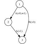
| state | A-1,-1 | A-1,0 | A-1,1 | A0,-1 | A0,0 | A0,1 | A1,-1 | A1,0 | A1,1 | B-1 | B0 | B1 |
| 1 | - | - | - | - | - | 2 | - | - | - | - | 3 | - |
| 2 | - | - | - | - | - | - | 3 | - | - | - | - | - |
| 3 | - | - | - | - | - | - | - | - | - | - | - | - |
GAL’s selection mechanism. GAL uses a torus to store the instances (a table that wraps around on the borders). In each step of the search, each instance may have a cross-over with randomly selected neighbors (among the eight adjacent neighbors of a cell in the torus). If the fitness of the child is better than the parent, it replaces the parent. Alternatively, the instance can be mutated (instead of the cross-over). Again, only a fitter instance will remain. This selection mechanism slows down the advance of fitter instances into the pool, allowing a search on several parts of the error surface simultaneously, without quickly getting stuck into local minima.
GAL’s cross-over operator. GAL introduces the FPU_cross-over (fitness proportional uniform cross-over) where a percentage (dictated by their relative differences in fitness) of the transition table from each parent is copied into the child. FPU_cross-over is a general GA operator, with a number of experiments justifying its advantages for the learning of automaton case.
GAL’s mutation operator. GAL mutation operator will flip positions in the transition matrix, respecting the number of states and depending on some parameters.
Stopping criteria. I use as stopping criteria reaching a maximum number of generations.
Initial population. The initial population is created by randomly choosing a number of states and variables and mutating every position in both the transition and variables matrices.
To tell good schema from bad ones implies in this case differentiating how well a proposed schema explains the training data. That is, a function that approximates the conditional probability of the schema S given the text T and knowledge K:

Actually, as I am searching for the best schema (S*) that maximizes this probability, I change my definition of the problem to use a likelihood:

From T and K, I can compute the relevant knowledge pool K′, a set of order constraints
and the sequence of atomic values Σ in an unsupervised manner, as described in the previous
section. My fitness function (similar to a likelihood in the context of a stochastic search) will
thus be defined as:
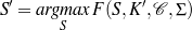
The hope is that S* and S′ will be the same or very close. To compute the function
F (S,K′,,Σ), I use the following heuristic definition, where I divide the fitness function into
three additive components, D are the document plans and Σset are the sequences of sets of
atomic values derived from D (in a process detailed below):
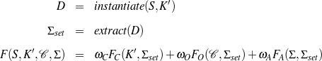
An important point to note here is that each of these three tiers are data-dependent as they analyze the goodness or badness of output document plans D, i.e., sequences of communicative predicates. They require instantiating the schema multiple times for each of the different knowledge sets K′. The document plans D are sequences of messages as the ones shown in Figure 5.2. These messages contain atomic values that can be extracted from them. However, the atomic values inside a message are unordered (the order is given later by the surface realizer). The extract function will keep them unordered, returning a sequence of sets Σset, where each set represents all the atomic values contained in a message (as a set so no assumptions are made with respect to their ordering). To make them compatible with sequence of first mentions, every repeated value is removed from the sets (i.e., also contain only first mentions). I combine the three functions with weights ωi, on the basis that, for example, a schema with great ordering but some mis-selections should not be discarded.
I will now analyze each tier in turn.
First Tier. The function FC(K′,Σset) measures the Content Selection in place (as opposed to the previous chapter, where no context was taken into account). The selected atomic values are extracted from the sequence of sets Σset and the FC is then the Fα measure described in the previous chapter, using α = 1 (precision is now considered as important as recall).
Second Tier. The second tier, FO, uses the order constraints mined over sequence of atomic values as described in Section 5.3.2.
Third Tier. The last component of the fitness function is its most interesting sub-function and the main contribution of my work. It compares the sequence of atomic values Σ with the sequence of sets of atomic values Σset (coming from the messages) by means of an alignment-based metric efficiently computed using dynamic programming.
This function scores how well the sequence of a set of atomic values Σset can be mapped into the sequence of atomic values Σ. This mapping is by virtue of non-crossing alignments between atomic values and sets of atomic values. This non-crossing property penalizes changes in ordering (i.e., when aligning A–B–C and C–B–A they will align both Bs but neither A nor C9) while enabling the use of dynamic programming, thus making this computation very efficient.
My dynamic programming is similar to global alignment with affine gap penalty, the Needleman–Wunsch algorithm in bioinformatics, as defined by (Durbin et al., 1998) (pages 17–28). The dynamic programming is governed by the following recurrences:
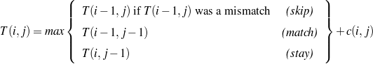
where c(i,j) is the comparison between a set of atomic values s at position i and an atomic value v at position j, it equals to 1 if the value is in the set and -1 otherwise:
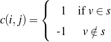
These recurrences can be understood as follows: at any given time during the alignment process, the alignment of the set of atomic values at position i (coming from the message) against the atomic value at position j equals the maximum of three possible values. The first value is that of an alignment skipping the previous set of atomic values (a skip). This option is only possible if the previous set of atomic values mismatched the atomic value (otherwise an atomic value will be double counted). Another possibility is that the previous atomic value matched successfully to the previous message (a match). Finally, several atomic values may be aligned to the same set of atomic values (the stay). In either case, the value of the alignment at that point is 1 if the atomic value belongs to the set or -1 otherwise.
Example:
Alignment of ![[A, B,C,D, E,F, G]](thesis191x.png) against
against ![[{B, C,D },{E, A},{C, B} ,{A, F} ]](thesis192x.png) . The
dynamic programming matrix will be:
. The
dynamic programming matrix will be:
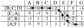
The alignment reads:
| A,B,C,D | E | F,G |
 |  |  |
Analysis. This fitness function so defined has a number of advantages. First, the degree of generalization in the schemata can be achieved by restricting the number of nodes available for the automata (to avoid memorizing the training material). Second, the incorporation of a Content Selection tier FC allows for a two level Content Selection learning where the fine grain Content Selection is performed in-place. That is the case because a complete Content Selection system can only be evaluated over the document plan, as a result of the inclusion of intermediate information following cohesion principles. Therefore, while the Content Selection rules mined in the previous chapter are of coarse granularity, fine Content Selection granularity can be adjusted at the schemata level. An important point to note here is that all three functions are data-dependent, as they analyze the goodness or badness of instantiated schemata. An advantage of the function FO is that while an aligned corpus is needed to collect the constraints, I consider the constraints to be valid for any knowledge so the constraints can be checked on a much larger range of semantic inputs,10 not only the ones used to mine the constraints. While FC measures content with no ordering and FA measures ordering in a very strict fashion, FO is somewhat in between. The contribution of FO is expected to be greater in earlier stages of the search, where the schema is producing results of too low quality to be fully evaluated using alignments. For example, let’s suppose the system is trying to learn ABCD and it is currently producing CDAB. Non-crossing alignments will be able to see that AB is correctly placed or CD is correct, but not both. For the sake of discussion, let’s say it aligns correctly CD:
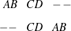
This alignment misses the important fact that AB is in the right order, that is, it will score CDAB the same as CDBA. Order constraints remedy that situation, allowing the system to reward differently instances that produce promising sub-sequences.
Finally, texts governed by DCK are supposed to be historically motivated, in the sense that their current shape does not necessarily obey any logic behind it, but there is a history of logically motivated changes that determine its current, accepted shape. Therefore, it may be the case that genetic algorithms can simulate that previous history.
I have investigated possible variations to the process described in this chapter (Duboue and McKeown, 2002). In particular, for the experiments in the medical domain discussed in the next chapter, I did not have enough data to perform an unsupervised step. Instead, a laborious manual tagging transformed the text side of the Text-Knowledge corpus in a sequence of message-types (semantic tags). However, this process could only be performed for a small number of texts. I succeeded in applying my technique in this different setting, with the following modifications:
Simpler schema. In this context, I targeted learning the schema-like planners discussed in the Related Work chapter, Section 2.2.1. These planners are schemata containing only sequence nodes and where each predicate has a Kleene star node preceding it.
No Content Selection. The data that should appear in the text was already selected. Moreover, the simpler schema did not allow for any Content Selection logic to be added to it. In a sense, it was using no focus decoding (greedy decoding).
Manual mapping of predicates to message types. The tag-set used by the tagging crew was developed by a domain expert and did not correspond directly to the system’s ontology, nor the existing schema predicates. I manually mapped one onto the other.
Text-to-text comparison. The most innovative variation was the use of a text-to-text comparison between generated text and the text part of the Text-Knowledge corpora. For computing the fitness function, I introduced the multiple-tiers approach described in this chapter, where the knowledge is used to produce document plans that are then scored for goodness. I scored them using order constraints in the same vein of the second tier of the fitness functions described in this chapter. From there, however, it was impossible to continue at the document plan level: the tagged texts did not contain information about the parameters that instantiated the predicate, only its type (e.g., I knew that an anesthesia predicate has been instantiated, but I lacked the information of which drug was given, and in which quantity —the parameters of the anesthesia predicate). The tagging crew did not annotate this information because it was present in the text inside the tag. To solve this problem, I employed the anchors hypothesis of my research11 and used the existing text generator to produce full verbalizations of the document plans (Figure 5.11). I then compare the generated text against the text from the Text-Knowledge corpus using a dynamic programming based function similar to the one described for the third tier of the fitness function presented in this chapter (but operating at the word level instead of the conceptual level). As substitution metric, I employed the information content on a corpus of related discourse.12
I evaluate the learned schemata by using hand tagged reference sequences of atomic values and computing the Kendall’s τ (Lebanon and Lafferty, 2002) as employed by (Lapata, 2003):

Where N is the number of objects (atomic values) and inversions is the number of exchanges on consecutive objects required to put them in the order appearing in the hand tagged reference. Because the sequence being evaluated is a sequence of sets of atomic values, for the sake of evaluation I consider the items inside the set are ordered in the correct order.
A schema is a highly structured representation, consisting in turn of a finite state machine, a set of rhetorical predicates and a focus decoder. The technique presented in this chapter targets the learning of the finite state machine given a set of rhetorical predicates and (McKeown, 1985)’s original focus decoding. The next two chapters present the results of applying this technique to two domains, medical and biographical. These chapters stress the contributions of the proposed fitness function and the mining of order constraints.
| Threshold | Description | Value |
| support threshold | Minimum number of sequences a pattern should
match to be further considered (this threshold is
expressed as percentage of the total number of
sequences). | 30% |
| throc | Probability threshold for a given order constraint to
be further considered. | 0.98 |
| nv | Number of variables per type. | 2 |
| windowsize | How many items are used to build a pattern. | 8 |
relative distance
threshold | Clustering parameter when mining order constraints. | 0.1 |
probability
cut-point | Minimum probability for accepting a learned
constraint. | 0.99 |
This chapter describes my contributions to the MAGIC project (Dalal et al., 1996, McKeown et al., 2000);1 this project built a generation system that produced briefings of patient status after a coronary bypass surgery. Normal work-flow in the hospital requires a medical specialist to give a briefing to the Intensive Care Unit nurses and residents before the patient arrives at the ICU. This briefing is given by one of the residents who was present in the operating room. The generation system uses data collected from the machines in the operating room to generate a coordinated speech and graphics replacement presentation for the briefing, avoiding distracting a caregiver at a time when they are critically needed for patient care. Figure 6.1 shows an example of a data excerpt (a CLASSIC data file with 127 facts on average) and generated presentation.
For evaluation purposes, (McKeown et al., 2000) collected and transcribed 24 briefings that then were used, along with the admission note (the gold standard), to quantify the quality of MAGIC output (100% precision, 78% recall). Each report transcription was subsequently annotated with semantic tags as shown in Figure 6.2, on page §.
When comparing the system output and the briefings, it can be seen that there are quite a few differences among them. In particular, the briefings are normally occurring speech. Aside from being much more colorful than the system output, they also include a considerable amount of information not present in our semantic input. And there is also some information present in the system that is not being said by the doctors, for example, because at the time the briefing is given, data such as the name of the patient is available in paper format to the target audience.
The transcripts and the semantic inputs constitute an aligned Text-Knowledge corpus, albeit a very small one. The experiments in this chapter address the Document Structuring schemata part of this thesis, with modifications to deal with the small amount of data. My task was to learn a tree representing a planner that performs as well as the planner developed manually for MAGIC. To remedy the lack of training material, more human effort was employed. The fitness function discussed in the previous chapter had three components: Content Selection, order constraints and alignments. In MAGIC, the planner makes no Content Selection decisions, therefore the first tier is not used in the MAGIC domain. For the other two tiers, the obvious choice would have been to assemble the matched texts by hand. This option, however, was utterly laborious. A simpler task in the form of semantic tagging was preferred.2 While the semantically tagged texts are a weaker source of information than the matched texts, in this case they are of pristine quality, as they were hand-built. The tagged texts provide semantic sequences to mine order constraints as discussed in the previous chapter (Section 5.3).
For the third tier, I had available the full-fledged MAGIC system. I combined the verbalize-and-search process from Chapter 3 with an alignment-based metric similar to the one presented in Chapter 5. For this combined metric, the MAGIC system produces a text presentation for the output (document plan) of the schemata being evaluated and then the text presentation is fed into an alignment based metric now at the text level.3 I thus align human text against the generated text.
In this chapter, I first introduce the data (Section 6.1), and then two series of experiments: learning order constraints (Section 6.2) and learning MAGIC schema-like planners (Section 6.3).
(age-12865, c-measurement, (a-value, 38), (a-unit, "year")) maps to sentence 1 (b)
(ht-12865, c-measurement, (a-value, 175), (a-unitm "centimeter")) maps to sentence 1 (b)
(name-12865, c-name, (a-first-name, "John"), (a-last-name, "Doe")) maps to sentence 1 (b)
…
(received-BloodProduct1-12865, c-receive-blood-product, (r-arg2, BloodProcut1-12865), (a-dosage, Measure-BloodProduct1-12865)) maps to sentence 5 to last (b)
(BloodProduct1-12865, c-blood-product, (a-name, ‘‘Cell Savers'')) maps to sentence 5 to last (b)
(Measure-BloodProduct1-12865, c-measurement, (a-value, 3.0), (a-unit, ‘‘unit'')) maps to sentence 5 to last (b)
…
(a)
In the aforementioned evaluation,4 McKeown et al. equipped the resident with a wearable tape recorder to tape the briefings, which they transcribed to provide the base of the empirical data used in this chapter. They subsequently annotated the text with semantic tags as shown in Figure 6.2. The figure shows that each sentence is split into several semantically tagged chunks. They developed the tag-set with the assistance of a domain expert in order to capture the different information types that are important for communication in this domain. Two non-experts did the tagging, after measuring acceptable agreement levels with the domain expert (McKeown et al., 2000). The tag-set totalled over 200 tags. The domain expert also mapped these 200 tags to 29 categories, which are the ones I used for my experiments.
From these transcripts, I derived the sequences of semantic tags building semantic sequences as the ones mentioned in the previous chapter (Figure 6.3). These sequences constitute the input and working material for my order constraints analysis, they have an average length of 33 tags per transcript (min = 13, max = 66, σ = 11.6). A tag-set distribution analysis (Table 6.1) showed that some of the categories dominate the tag counts (this is similar to the effect seen by (Varges, 2003) when semantically tagging leading sentences in WSJ acquisition articles). Furthermore, some tags occur fairly regularly towards either the beginning (e.g., date-of-birth) or the end (e.g., urine-output) of the transcript, while others (e.g., intraop-problems) are spread more or less evenly throughout.
Obtaining these transcripts was a highly expensive task involving the cooperation and time of nurses and physicians in the busy ICU. My corpus contains a total number of 24 transcripts. Therefore, it was important to develop techniques that can detect patterns without requiring large amounts of data.
| tag name | count | ||||
| allergies | 20 | 40 | 50 | 10 | |
| blood-gases | 2 | 100 | |||
| cardiac-output | 30 | 3 | 7 | 30 | 60 |
| cell-saver | 21 | 5 | 43 | 52 | |
| cross-clamp-time | 10 | 40 | 40 | 20 | |
| date-of-birth | 13 | 100 | |||
| drip | 42 | 10 | 60 | 31 | |
| exogenous-red-blood-cell | 12 | 42 | 58 | ||
| fluid | 33 | 3 | 52 | 45 | |
| height | 5 | 100 | |||
| h/h | 21 | 5 | 9 | 33 | 52 |
| intubation | 34 | 21 | 62 | 12 | 6 |
| intraop-problems | 92 | 4 | 25 | 45 | 26 |
| labs | 17 | 6 | 29 | 65 | |
| minute-bypass-time | 11 | 55 | 27 | 18 | |
| name | 6 | 100 | |||
| operation | 27 | 37 | 44 | 19 | |
| other-lines | 10 | 20 | 80 | ||
| platelet | 2 | 100 | |||
| preop-diagnosis | 18 | 94 | 6 | ||
| past-medical-history | 154 | 75 | 16 | 7 | 2 |
| preop-med | 96 | 36 | 59 | 1 | 3 |
| sex | 9 | 100 | |||
| swan | 5 | 20 | 80 | ||
| temperature-intraop | 2 | 50 | 50 | ||
| total-meds-anesthetics | 79 | 23 | 59 | 18 | |
| urine-output | 17 | 24 | 76 | ||
| weight | 5 | 80 | 20 | ||
As explained in Chapter 5, learning order constraints is a case of unsupervised learning: sets of patterns, clusters of patterns and order constraints over clusters are mined from the sequences of semantic tags without any need of annotated data. To test the quality of the acquired patterns, clusters and constraints, I keep aside a set of held-out semantic sequences and compute how often the patterns identified during training can be identified in the held-out; how often clusters of patterns can be identified, and, more interestingly, how often the order constraints do hold over the held-out sequences, using the metrics introduced in Section 5.3.2. I will present quantitative results using them via cross validation. A comparison against the plan of the MAGIC system for qualitative evaluation closes this section.
I used 3-fold cross-validation to compute these metrics averaged over 10 executions of the
experiment. The different parameter settings were defined as follows: for the pattern detection
algorithm, I set  to
to  (a window size of 8) and the support threshold to 0.2. The
clustering algorithm used a relative distance threshold of 0.1. The results at the probability
cut-point of 0.99 are reported below. This figure was chosen to avoid generating a very large
number of constraints.
(a window size of 8) and the support threshold to 0.2. The
clustering algorithm used a relative distance threshold of 0.1. The results at the probability
cut-point of 0.99 are reported below. This figure was chosen to avoid generating a very large
number of constraints.
The system obtained an average of 58.538 (±8.460) patterns,5 clustered into 19.705 (±3.023) clusters. When tested on the held out fold, all patterns and clusters are found. For the default cut-point of 0.99, an average of 401.938 (±51.226) constraints are found,6 from which 205.205 (±45.954, a 51.904%) are always correct, 196.605 (±68.134, a 48.072%) sometimes contain errors and 0.138 (±0.350, a 0.037%) contains a large number of errors. Table 6.2 shows other results at different probability cut-points.
| cut-point | found | valid | mixed | invalid
| ||||||||
| 1 | 30.71 | ± | 7.56 | 8.55 | ± | 6.68 | 22.21 | ± | 8.62 | 0.00 | ± | 0.00 |
| 0.99 | 401.98 | ± | 51.27 | 205.25 | ± | 45.99 | 196.65 | ± | 68.17 | 0.18 | ± | 0.39 |
| 0.98 | 461.88 | ± | 59.97 | 240.35 | ± | 50.83 | 221.28 | ± | 77.44 | 0.35 | ± | 0.75 |
| 0.97 | 465.25 | ± | 60.34 | 240.35 | ± | 50.83 | 224.65 | ± | 77.66 | 0.35 | ± | 0.75 |
| 0.9 | 606.01 | ± | 74.96 | 329.91 | ± | 63.86 | 274.81 | ± | 93.31 | 1.38 | ± | 1.65 |
| 0.8 | 712.48 | ± | 82.47 | 397.58 | ± | 73.2 | 311.98 | ± | 101.48 | 3.01 | ± | 2.44 |
| 0.7 | 831.75 | ± | 93.33 | 490.51 | ± | 85.54 | 336.48 | ± | 108.81 | 4.85 | ± | 300 |
Figure 6.4 shows the impact of the support threshold. As we require the patterns to appear in more instances in the training set, less patterns are found, which in turn produce clusters and constraints with higher accuracy. A support threshold of 0.2 seemed a good compromise between the number of patterns and their quality.
Figure 6.5 illustrates the effect of the window size on the different metrics. As the window size grows, better quality is achieved. The curves stabilize at a window size of 8, the number employed in my experiments.
Figure 6.6 shows the impact of the distance threshold for clustering. While fewer clusters may arguably produce better results, I settled for a small distance threshold to obtain a greater number of clusters and therefore be able to appreciate the effects of clustering better.
The learning curve (Figure 6.7) shows some of the problems of working with such a small data set: the curves present some peaks and valleys and still shows no sign of stabilizing.
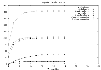
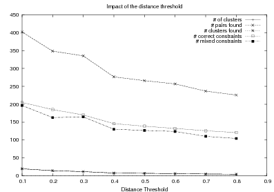
The system was executed using all the available information (the 24 transcripts), with similar parametric settings to the ones used in the quantitative evaluation, yielding a set of 29 constraints, out of 23 generated clusters.
These constraints were analyzed by hand and compared to the existing strategic component. We found that most rules that were learned were validated by the existing plan. Moreover, we gained placement constraints for two pieces of semantic information (e.g., medical history) that are currently not represented in the system’s plan. In addition, we found minor order variation in relative placement of two different pairs of semantic tags. This leads us to believe that the fixed order on these particular tags can be relaxed to attain greater degrees of variability in the generated plans. The process of creation of the existing content-planner was thorough, informed by multiple domain experts over a three year period. The fact that the obtained constraints mostly occur in the existing plan was very encouraging.
The framework described in Chapter 5 (Section 5.5) was implemented as follows: I employed a population of 2000 chromosomes, discarding 25% of the worse-fitted ones in each cycle. The vacant places were filled with 40% chromosomes generated by mutation and 60% by cross-over. The mutation operator was applied with a 40% probability of performing a node insertion or deletion and 60% chance of choosing a shuffle mutation. The population was started from a chromosome with one root node connected to a random ordering of the 82 operators and then nodes were inserted and shuffled 40 times.7
As baseline, I used the initial population of the three runs (6K randomly built planners in total). The MAGIC planner was used as my gold standard, as it has been previously evaluated by domain experts as highly accurate and was not involved in my learning process at any part.
The planner used in the MAGIC system was developed with efficiency in mind, but it lacks flexibility and the plan used is more appropriate for textual output (as opposed to the speech output it was targeted). It has a total of 274 operators, 192 of them being structure-defining (discourse or topic levels) and 82, data defining (atomic level) operators.8 Figure planner, the input is checked for the existence of the datum specified by the operator. If there is data available, the corresponding semantic structures are inserted in the output.9 The internal nodes, on the other hand, form a tree representing the discourse plan; they provide a structural frame for the placement of the atomic operators. Thus, the execution of the planner involves a traversal of the tree while querying the input and instantiating the necessary nodes (an example of such trees was presented in Chapter 2, Figure 2.5).
The MAGIC strategic component uses a tree as internal representation because its document plans contain text planning information (i.e., top level nodes provide paragraph divisions) and aggregation information (the elements below pre-terminals can all be aggregated together). If it not were for this extra information, a plain sequence of atomic operators would be equally expressive. On the other hand, I expect the genetic algorithm handling of the trees to produce robust structures: only pre-terminals that behave reasonably well under node shuffling mutations will remain in the genetic pool, meaning that trees with felicitous arranging of the internal nodes will increase their presence in the population.
The MAGIC generator has a special emphasis on its aggregation component, Casper (Shaw, 2001). One of the original motivations of my proposed architecture was to learn automatically the interaction between the planner and the aggregation component. While my preliminary experiments (Duboue and McKeown, 2002) showed the feasibility of such approach, it had two drawbacks: first, it requires the MAGIC generator to be effectively run for every document plan. If aggregation is disable, the caching mechanism described below can be employed to dramatically speed up the approach. The second drawback is more problematic to the experiments presented here; Casper imposes a number of preconditions on the strategic component. If these preconditions are not satisfied, its behavior is undefined. Because the existing planner satisfies these preconditions, including the aggregation component into the fitness function adds an extra piece of information to the function, biasing the function towards the MAGIC planner. This situation is problematic, as I am interested in analyzing the feasibility of reproducing the existing planner using only the Text and Knowledge corpus.
When the aggregation component is switched off, every atomic operator will ultimately produce a sentence on its own. The quality of the generated text will be then quite low and very repetitive (repeating phrases such as the patient is in almost half of the sentences and so on). This repetitive nature should not be a major problem as the text-to-text metric employs the word information content computed over a large corpus of comparable texts to score the relative importance of words.
I evaluate using the Kendall’s τ described in the previous chapter:

Where N is the number of objects (atomic operators) and inversions is the number of exchanges on consecutive objects required to put them in the order returned by the MAGIC planner.
I did a number of experiments to gain further insights on the search process and validate the approach. For the first experiment, I looked to build a characterization of the search process. To that end, I let the search go for 50 iterations, in one run. The fitness of the best instance is plotted in Figure 6.8. The search achieves a certain level of stabilization around iteration 25. I thus plot three different runs (together with an interpolated average) until iteration 21 (Figure 6.9) to validate the learning process.
Another way to appreciate the learning process is to take a look at the goodness of the population as a whole, at different generations (Figure 6.10). There we can see that the order constraints are important at early stages of the search.
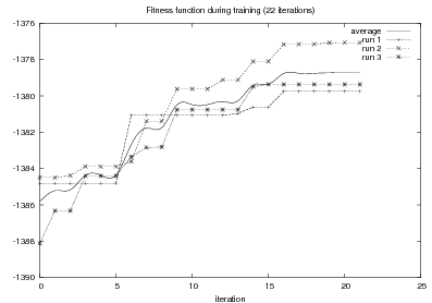
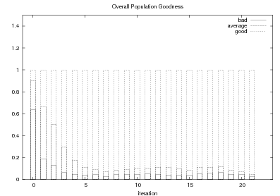
The second experiment is the actual evaluation of the planners against the MAGIC planner, using Kendall’s τ. In this experiment, three independent runs are iterated 21 steps. The best instance for each run at each iteration step is executed over 50, unseen, semantic inputs and the output document plan (converted into a sequence of atomic operators) is scored against the sequence obtained from the MAGIC planner. The average over the three runs gave τ of 0.2288 ± 0.0342.
To provide a baseline, I joined together the first generation of the three runs (a total of 6,000 random instances). When scored using Kendall’s τ against the MAGIC planner, they had an average τ of 0.0952 (± 0.1144).
These experiments show the feasibility of the approach, although the training material was unsuitable to fully re-create the existing MAGIC planner. It would have been interesting to see the impact of the technique as a quick prototyping tool during early stages of the development of the project, although that is no longer possible.
This chapter exemplifies the application of the technique described in the previous chapter to data in the medical domain. This domain has a straightforward rhetorical structure that allows my techniques to positively learn Strategic Generation logic.
From a broader perspective, the results are quite low. A τ of 0.22 shows an improvement over a completely random baseline but it is still a weak correlation with the MAGIC planner. I think the problem in this case is to evaluate the automatically obtained schema against the MAGIC planner. It may be the case that the training material differs to a large extent with the MAGIC planner.10 Moreover, the reduced training size forbids using cross-validation techniques to analyze how well the learned planners perform when tested against unseen training material.
The approach presented here is definitely CPU-intensive with running times usually expressed in days. Nevertheless, as Figure 6.9 shows, this is a search process that makes positive progress towards its goal. Moreover, the progress is not only in the best instance of the population, but it is a progress across the board, as shown in Figure 6.10, where it is clear that as times progresses, the population contains a larger percentage of really worthy instances. This progress is to be contrasted with the lack of progress when these technique are applied to ProGenIE data, as presented in the next chapter.
Figure 6.10 also shows the impact of the order constraints, as earlier stages of the population use them to distinguish totally wrong instances (the lower part of the bar) with the most promising instances (the upper part of the bar). Other extrinsic evaluations of the value of the order constraints were not attempted.
Contrasting MAGIC and ProGenIE results, it begs the question of which attributes in the MAGIC data makes it amenable for the learning. As mentioned in Chapter 2 (Section 2.2.1), MAGIC schemata are only suitable for planning single-topic discourse, as all discourse in MAGIC has the same focus —the patient the surgery was about. In the ProGenIE data, for the contrary, the focus shifts from the actor being described to her selected movies, and then to major awards each movie itself received.
(a)
This chapter describes the second round of Document Structuring experiments performed in this dissertation. As part of the joint Columbia University—University of Colorado Open Question Answering project (AQUAINT), I developed ProGenIE, a biography generator. The goal of ProGenIE was to provide final users with means to quickly and concisely communicate information about persons of interest. I combined a natural language generator with an information extraction infrastructure leading to ultimately mix textual (such as existing biographies and news articles) as well as non-textual (such as airline passengers lists and bank records) sources. I used the examples from the domain contained in the corpus described in this chapter to automatically construct Document Structuring schemata. These schemata guide the generation of biographies on unseen people.
I gathered an aligned Text-Knowledge corpus in the biography domain, as explained in the next section. More specifically, my corpus is a collection of human-produced texts together with the knowledge base a generation system might use as input for generation. The knowledge base contains many pieces of information related to the person the biography talks about (and that the system will use to generate that type of biography), not all of which necessarily will appear in the biography. That is, the associated knowledge base is not the semantics of the target text but the larger set1 of all things that could possibly be said about the person in question. The ordering of the intersection between the input knowledge base and the semantics of the target text is what I am interested in capturing by means of my statistical techniques.
The Text-Knowledge corpus used in this chapter consists of knowledge’s extracted from a semi-structured knowledge, biographical fact-sheets of assorted celebrities. These fact-sheets were crawled from E! on-line2 in November 2002. In addition to this knowledge source, I also employ an extended knowledge source, also extracted from E! on-line but with a slightly different ontology and with information about the movies actors appeared in added. This extended knowledge knowledge source was incorporated to these experiments at the end of this dissertation and was not used during system development. Different biographical sites provide the text part, to test the ability of the system to learn from different types of data. As explained in Section 3.2.1, each corpus was split into a training and test set, with the test set tagged for selection and ordering (ordering only in the last corpus) by the author.
The annotation was done by the author, by reading the biographies and checking which
triples (in the RDF sense, 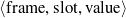 ) were actually mentioned in the text (going back
and forth to the biography as needed). Two cases required special attention. The first one was
aggregated information, e.g., the text may say “he received three Grammys” while in the
semantic input each award was itemized, together with the year it was received, the reason and
the type (Best Song of the Year, etc.). In that case, only the name of award was selected, for
each of the three awards. The second case was factual errors. For example, the biography may
say the person was born in MA and raised in WA, but the fact-sheet may say he was born in
WA. In those cases, the original aim of the human writer was given priority and
the place of birth was marked as selected, even though one of the two sources were
wrong.
) were actually mentioned in the text (going back
and forth to the biography as needed). Two cases required special attention. The first one was
aggregated information, e.g., the text may say “he received three Grammys” while in the
semantic input each award was itemized, together with the year it was received, the reason and
the type (Best Song of the Year, etc.). In that case, only the name of award was selected, for
each of the three awards. The second case was factual errors. For example, the biography may
say the person was born in MA and raised in WA, but the fact-sheet may say he was born in
WA. In those cases, the original aim of the human writer was given priority and
the place of birth was marked as selected, even though one of the two sources were
wrong.
Biographical Descriptions Domain. Biography generation is an exciting field that has attracted practitioners of NLG in the past (see the Related Work chapter, Section 2.4.3). It has the advantages of being a constrained domain amenable to current generation approaches, while at the same time offering more possibilities than many constrained domains, given the variety of styles that biographies exhibit, as well as the possibility for ultimately generating relatively long biographies.
The AQUAINT project focuses mostly on military and intelligence targets. However, there is a lack of publicly available information about such targets. Therefore, I shifted my attention to more popular individuals. As my approach is based on Machine Learning, given enough training data, the particular biographical field chosen is immaterial.
By far the most popular domain for biographies and assorted data about people is the celebrities domain. Most fans are eager to express their support to their favorite actor, model, singer or director by collecting sizable amounts of trivia or assembling them in very detailed biographies. The availability of information in this domain has lured other researchers into working with it (Pang et al., 2002, Taskar et al., 2001).
I obtained the semantic input from pages describing itemized factual information about persons: fact-sheet pages (Figure 7.1). Such pages are abundant for celebrities (singers, movie stars and other famous people).
However, the level of detail of the fact-sheets was too coarse for my needs; I employed a combination of Information Extraction (IE) scripts to break the fact-sheet pages into smaller parts. A full-fledged natural language generation system expects a level of detail in its input that goes beyond the lay person ontological modeling found in the mined fact-sheets. To improve over that scenario, I performed a process I termed Closed Information Extraction. In this process, I build scripts without generalization in mind. It can be thought of as over-fitting a regular IE process.
My current corpus contains semantic information for about 1,100 people, together with aligned biographies in four different sub-corpora, linked against 108, 578, 205 and 341 biographies for each of these sub-corpora. The sub-corpora were mined from four different Web sites and contain different writing styles and text structure. Such an environment is ideal for learning and testing content planning related issues.
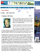 | 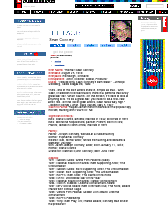 |
| (a) Biography | (b) Fact-sheet |
The acquisition process consisted roughly of three steps: crawling, cleaning and linking. The crawling step involved downloading the actual pages. The cleaning step was the most time-consuming step and involved the Closed Information Extraction process mentioned above. Finally, I had data about people and biographies about (hopefully the same) people. The last step took care of linking data with biography, when appropriate.
While E! Online contains also biographies, chances are the fact-sheets are based on the biographies or vice-versa. To improve the quality of the aligned corpora, I mined different sites for the biographies. While several Web sites offer biographical information repositories, most of them focus in particular type of individuals. The sites I crawled that made up my corpus are: www.biography.com, www.s9.com, www.imdb.com, and www.wikipedia.org.
| Agency | Education |
| Awards | Factoids |
| Birth date | Family |
| Birth Name | Occupations |
| Birthplace | Person |
| Claim to Fame | Quote |
| Date of Death | Significant Other(s) |
Regarding the cleaning step, it was the most time-consuming step, as already mentioned. This was no surprise, as data cleansing is normally considered among the most time consuming steps in data mining (Rahm and Do, 2000).
I cleaned the fact-sheets by means of a Closed Information Extraction process. The fact-sheets originally contained information in 14 categories, shown in Table 7.1. While some categories contained information that could be directly included in my knowledge representation (I use a representation similar to RDF (Lassila and Swick, 1999)), others contained heavily aggregated information (some difficult cases are shown in Figure 7.2).
To cope with these cases, I wrote a series of scripts, with patterns to capture different types of information. As usual, the patterns had errors, most frequently over-generating.
Having a sizable set of semantic inputs and several sets of biographies as separated resources involved a real problem when it was the time to put them together. While I did not hesitate in spending hours of human labor for the construction of this corpus, aligning 1,100 fact-sheets against 20,000 biographies is truly unfeasible to be done by hand. I thus needed to link the two resources, a step complicated by the fact that names tend to be paraphrased, and are not unique identifiers (e.g., there is a silent-movies era actor also named Harrison Ford). I used techniques from record linkage in census statistical analysis (Fellegi and Sunter, 1969), a well studied discipline with more than 40 years of practice.
This section summarizes major highlights of the constructed corpus. I briefly describe the knowledge representation, and report total figures of frames, relations, words, tokens and links.
I employed a type-based frame structure, with inheritance. The information for each
person is kept in a separate file, as a set of frames. Each frame has a unique name, a type
(linked to an ontology) and a list of attribute-value pairs. Following RDF nomenclature, I count
triples of the form  . Attributes can be list-valued, can refer to
other frames, or may contain atomic values (currently of types symbol, string, or
number).
. Attributes can be list-valued, can refer to
other frames, or may contain atomic values (currently of types symbol, string, or
number).
The final corpus contains 50,000 frames, with 106K frame-attribute-value triples, for the 1,100 people mentioned in each fact-sheet. The frames are linked through 43 different relations shown in Table 7.2. An example set of frames is shown in Figure 3.1.
agency aka award birth canned-text city claimtofame country date day death degree education end factoids | father first full givenname last major month mother name occupation older place postmod premod | province quote reason relative significant-other source start subtitle teaching-agent text title xtra year younger |
The details of the linked resource were detailed in Chapter 3, but I summarize their details in Table 7.3.
| biography.com | Total | Average | Train | Test
|
| # pairs | 102 | - | 91 | 11 |
| # frames | 4,956 | 45.588 | 4,442 | 514 |
| # triples | 10,628 | 104.196 | 9,500 | 1,128 |
| # words | 54,001 | 529.422 ± 301.15 | 49,220 | 4,781 |
| # chars | 337,775 | 3,311.520 ± 1,857.96 | 307,978 | 29,797 |
| s9.com | Total | Average | Train | Test
|
| # pairs | 578 | - | 558 | 20 |
| # frames | 30,709 | 53.130 | 29,723 | 986 |
| # triples | 95,032 | 164.415 | 92,969 | 2,063 |
| # words | 21,037 | 36.396 ± 34.04 | 20,192 | 845 |
| # chars | 138,711 | 239.984 ± 215.82 | 133,204 | 5,507 |
| imdb.com | Total | Average | Train | Test
|
| # pairs | 199 | - | 185 | 14 |
| # frames | 10,123 | 50.869 | 9,362 | 761 |
| # triples | 31,676 | 159.176 | 29,323 | 2,353 |
| # words | 64,196 | 322.593 ± 285.63 | 60,086 | 4,110 |
| # chars | 378,778 | 1,903.407 ± 1,693.88 | 354,560 | 24,218 |
| wikipedia.org | Total | Average | Train | Test
|
| # pairs | 361 | - | 341 | 20 |
| # frames | 58,387 | 161.737 | 55,326 | 3,061 |
| # triples | 108,009 | 299.194 | 102,297 | 5,712 |
| # words | 68,953 | 191.006 ± 55.17 | 64,784 | 4,169 |
| # chars | 418,035 | 1,157.992 ± 334.01 | 392,925 | 25,110 |
Mimicking the experiments in the previous chapter, the system obtained an average of 14.171 (±1.806) patterns, clustered into 3.838 (±0.384) clusters. When tested on the held out fold, all patterns and clusters are found. For the default cut-point of 0.99, an average of 537.038 (±18.426) constraints are found,3 from which 276.638 (±15.502, a 51.502%) are always correct, 260.405 (±12.377, a 48.507%) sometimes contain errors and no constraints contains a large number of errors. Table 7.4 shows other results at different probability cut-points. These figures are compatible with the ones presented in the previous chapter.
| cut-point | found | valid | mixed | invalid
| ||||||||
| 1 | 61.35 | ± | 3.82 | 24.85 | ± | 3.44 | 36.54 | ± | 4.58 | 0.00 | ± | 0.00 |
| 0.99 | 537.08 | ± | 18.47 | 276.68 | ± | 15.54 | 260.45 | ± | 12.42 | 0.00 | ± | 0.00 |
| 0.98 | 598.94 | ± | 20.13 | 306.01 | ± | 15.95 | 292.95 | ± | 13.78 | 0.08 | ± | 0.23 |
| 0.97 | 605.41 | ± | 20.24 | 306.01 | ± | 15.95 | 299.41 | ± | 14.44 | 0.08 | ± | 0.23 |
| 0.9 | 766.65 | ± | 27.49 | 403.41 | ± | 21.4 | 363.21 | ± | 15.11 | 0.11 | ± | 0.41 |
| 0.8 | 930.81 | ± | 30.79 | 497.81 | ± | 24.58 | 432.88 | ± | 13.98 | 0.21 | ± | 0.51 |
| 0.7 | 1134.01 | ± | 37.61 | 668.58 | ± | 30.49 | 465.14 | ± | 17.72 | 0.38 | ± | 0.65 |
Figure 7.3 shows the impact of the support threshold. Again, as we require the patterns to appear in more instances in the training set, less patterns are found, which in turn produces clusters and constraints with higher accuracy. Here too, a support threshold of 0.2 seemed a good compromise between the number of patterns and their quality.
Figure 7.4 illustrates the effect of the window size on the different metrics. As the window size grows, better quality is achieved, but the window stabilizes very early in the process.
The learning curve (Figure 7.5) shows that the training material is now enough to produce a smooth curve.
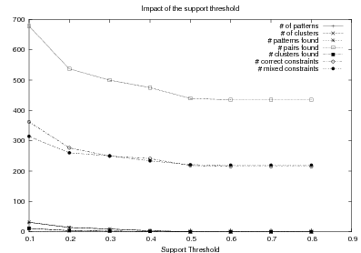
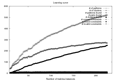
I will discuss here my preliminary results in learning Document Structuring schemata. I fully implemented the approach described in Chapter 5 and performed a number of rounds of training with the order sequences obtained from the Variant 4 matched texts in the wikipedia.org corpus. Figure 7.6 shows one such a run, representative of the experiments I conducted. The figure shows the evolution (or lack of it) of the fitness function. Even though my approach is faster than doing full verbalization, the curve took a good one week to be computed on a dual 3Ghz Pentium 4 machine. The curve shows a certain improvement over time, however (the peak around iteration 300). This very slow rate of convergence can easily be attributed to two factors: the size of the search space and the lack of training-motivated operators. While the fitness function is defined by the training material, the operators just induce random alterations on the instances (schemata). Given the size of the search space this ensures a particularly slow convergence for the search.
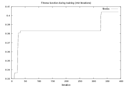
A schema at the end of the process is shown in Figure 7.7. This figure may be a piece of evidence for another problem with the approach: the focus mechanism is an integral part of the semantics of the schemata. Without a deep understanding of both the meaning of the communicative predicates (the edges in the graph) and the prioritization made by the focus mechanism, it is very difficult, if not impossible to predict the path over the graph that will result in the document plans. I suspect the focus mechanism as defined originally by (McKeown, 1985) is hurting my learning, because it can result in abrupt changes on the schemata. It seems learning both items together will benefit the composite process.
The domain of biographical descriptions contains some of the complexities that makes the Strategic Generation problem difficult in a general setting (recursion, branching, etc.). These complexities imply further research is needed to fully acquire a schema from a Text-Knowledge corpus. This subject is further explored in the next chapter.
Continuing with the discussion in the conclusions of the previous chapter, here a complex domain implies a domain that requires to drill down in different entities. The example biography schema, shown in Figure 5.3, contains many such drill downs: for example, after an entity (built) of which the person (Self) has been involved into the construction has been introduced, the appraisals motivated by that entity are enumerated.
The difference then between the MAGIC data and the ProGenIE data is in the latter’s need to capture focus shifts during learning. The hope was that, as the technique described in Chapter 5 was focus agnostic, the GA was going to be able to learn the schema in spite of this focus problem.
Sadly, post hoc analysis shows that focus affects the GA too negatively; when a very promising solution is slightly modified, most of the time it will produce a completely invalid offspring. That means that, for the most part no improvements are done in each step of the genetic search. This can be seen by comparing Figure 6.9 in the previous chapter with Figure 7.6. Both figures took comparable amount of time to be computed. We can see that in roughly the same amount of time, the approach without using verbalizations takes an order of magnitude less time to compute. However, in 21 steps the system running in MAGIC data already stabilizes. In 392 steps, the system running in ProGenIE data has managed to make only one successful step. Moreover, it is intuitive that the ProGenIE data will need more than only 21 steps to find a solution. Therefore, if it takes about a week to do each of these steps, it is clear that the current solution runs into computational feasibility problems with this data.
With respect to the order constraints, the lack of results in the overall schema learning forbids an extrinsic evaluation as done in the previous chapter. A feasible alternative would have been to evaluate their use as stand-alone planners, but this approach was not attempted.
Some ways to go around the problems identified in these experiments will be discussed in the next chapter and in the conclusions chapter. Succinctly, one alternative would be to improve the system with more informed operators that will modify the population according to the training material (data-driven operators). Another promising alternative is learning the focus mechanism together with the finite state automaton. Both approaches are target for future work.
My proposed technique to acquire Content Selection rules and Document Structuring schemata from a Text and Knowledge corpus has a number of drawbacks and limitations. I have identified some of them that I will summarize in this chapter. I will first discuss general limitations of my techniques (Section 8.1), including the need for a Text-Knowledge corpus and domain requirements. The limitations of the matched text construction process are discussed in Section 8.2. Finally, the learning of Content Selection rules and Document Structuring schemata have particular limitations discussed in Section 8.3 and Section 8.4, respectively.
I will now mention briefly some general limitations of my approach.
Knowledge requirement. The Strategic Generation component in a NLG system operates at a very high level of abstraction; it takes knowledge as input and produces document plans as output. It is natural that a system learning Strategic Generation logic will also require knowledge as training material. This requirement obviously restricts the application of the technique to domains where such structured knowledge can be gathered. Luckily, existing efforts such as the W3C Semantic Web (Berners-Lee et al., 2001) or the standardization of XML formats1 increase the availability of structured knowledge.
Text-Knowledge corpus requirement. This is a major requirement of my technique. In a sense, my thesis is an exploration of the possibilities of such a formidable learning resource. Working on relaxations to the Text-Knowledge requirement is an attractive follow-up to my work, for example using text alone and extracting knowledge from it by means of information extraction techniques. It would be difficult, if not impossible, to acquire Content Selection knowledge with such an approach. Other researchers have coped with the lack of a perfect Text-Knowledge resource with manual efforts. (Barzilay and Lee, 2002) had knowledge available and then had people write verbalizations for it. On the contrary, (Karamanis and Manurung, 2002) had texts available and built associated knowledge.
Domain Requirements. For a more precise description of the domain requirements imposed by my technique, five issues need to be taken into account:
There is a lack of intentional structure per segment of the text; from the intentional stand-point, the whole text is an atomic Intention: Report. Measuring this fact is quite complex but I would argue new techniques for opinion detection can be of use here (Taskar et al., 2001, Pang et al., 2002, Yu and Hatzivassiloglou, 2003).
Computationally Expensive. The methods employed in this thesis normally involve searches in large spaces and other computationally intensive tasks. This type of behavior is to be expected when dealing with large combinatorial problems. More importantly, most of the algorithms described here are parallelizeable with trivial or nearly trivial effort. Some of my experimental chapters also speak of the feasibility of my technique, although some of the problems in the previous chapter can be traced back to this limitation.
Learning for NLG. My work relates to recent uses of Machine Learning techniques for NLG tasks. A word of caution is required, as the type of logic produced will mimic the quality of the material offered to the system. (Reiter and Sripada, 2002) pointed out that exposing a learning system to poorly written text will learn a robust understanding system. In the NLG case, however, they pointed out that using poor texts will be akin to using poor parse trees in the understanding setting: poor training text means poor output text quality in NLG, not robustness. Moreover, I believe careful study of a domain allows the NLG practitioner to make a system that generates better texts than the average human. Humans do not succeed in producing texts that are consistent, unambiguous and concise at all times. A well tuned NLG system can reach such levels of perfection. By learning a symbolic representation, my thesis fits perfectly in this picture as a quick prototyping tool.
Thresholds and Parameters. The parameter tables in the different chapters (summarized in Table 1.1) point to another limitation of this thesis’ techniques: the need for a number of thresholds and parameters. This necessity arises from two sources. First, the use of a unsupervised learning approach in areas of this thesis usually calls for certain parameters to be hand-picked. This is normal practice in other unsupervised settings (e.g., the number of cluster in a clustering application). Second, Genetic Algorithms are usually criticized as having a number of parameters (e.g., population size, mutation rate, etc.) that varies widely from application to application of GAs. My particular deployment of GAs does not escape from this limitation.
The situation described above is a true limitation of the approach described here. Nevertheless, as explained in Chapter 1, I envision a Strategic Generation-learner system as a tool for the NLG practitioner that will assist the practitioner when building a NLG system for a new domain. As such, the parameters of this tool (my system) will have to be dealt intuitively by the NLG practitioner. The parameters I used in my experiments (shown in Table 1.1) are provided as a means to help build these intuitions.
The matched text construction process is a large source of errors but also a major contribution of this thesis. Unsupervised systems derive all their behavior from underlying assumptions on the model. This fact makes them unstable and difficult to deal with in general. My system is no exception to these general issues. To talk of its shortcoming is to talk about the shortcomings of the model itself. I will just point out two major issues I have noticed while experimenting with the approach: the need for large amounts of text and the fact that the system can be easily mislead.
Because of its statistical nature, large quantities of text are needed to identify
meaningful verbalizations. Moreover, even if normally the ‘default’ verbalizations are picked
by the system, an even larger amount of text is necessary to select relevant variants. In
experiments (unreported in this thesis) I have pursued using a 25M words corpus
downloaded from the Web, the system was able to identify ‘Johnny’, ‘J’ as possible
verbalizations of  . With a little more effort, I would expect the
system to identify ‘Dick’ as a verbalization for
. With a little more effort, I would expect the
system to identify ‘Dick’ as a verbalization for  . Now, it
would be definitely impossible to pick up a verbalization of ‘Pirot’ for the concept
. Now, it
would be definitely impossible to pick up a verbalization of ‘Pirot’ for the concept
 . However, humans will have no problem telling that (maybe not
proposing ‘Pirot’ as a verbalization of ‘Ipeirotis’ in abstract, but identifying in a given
text that ‘Pirot’ refers to the last name ‘Ipeirotis’ —context makes a big difference,
usually). However, there is no human intervention during the matched text construction
(again, it is unsupervised). Therefore, it needs a large number of textual examples
and even in that case there will be cases that cannot be captured. Note that this is a
problem with the model. The model, however, can be improved to accommodate new
cases.2
More research is needed to propose new models and enrich existing ones. Mine is a simple
model to help bootstrap the exploration process.
. However, humans will have no problem telling that (maybe not
proposing ‘Pirot’ as a verbalization of ‘Ipeirotis’ in abstract, but identifying in a given
text that ‘Pirot’ refers to the last name ‘Ipeirotis’ —context makes a big difference,
usually). However, there is no human intervention during the matched text construction
(again, it is unsupervised). Therefore, it needs a large number of textual examples
and even in that case there will be cases that cannot be captured. Note that this is a
problem with the model. The model, however, can be improved to accommodate new
cases.2
More research is needed to propose new models and enrich existing ones. Mine is a simple
model to help bootstrap the exploration process.
The matched text construction works on the hypothesis that changes in the data are correlated with changes in the text. There are times that the change in data affects the text, while not appearing explicitly. For example, on work on revision-based generation (Robin and McKeown, 1993), it was the case that information that did not appeared in the text was affecting lexical choice: stocks surge when they start raising in the morning but they raise if they do it in the middle of the day, although the actual time does not appear mentioned in the text.3 Therefore, keeping these concepts for further processing is of use for a NLG pipeline; as the example show, the data not selected for inclusion has a role in lexicalization. In any case, the overgeneration implies that the statistical rules will be prone to have low precision.
Inducing Content Selection logic from a Text-Knowledge corpus will capture paradigmatic, schema-like information that has to be included in the text. Capturing this paradigmatic information has been the objective of my work. However, it is clear that not all the information that makes up a text can be obtained this way: biographies, for example, will usually contain mentions to out-of-the-ordinary facts about a person that are worth being reported. Take again the MTV Movie Awards discussed in Chapter 4 as omitted in celebrities biographies. Now, if a person had won the MTV Movie Awards every year for the last ten years, such fact will be included in the biography. Techniques that operate exclusively on the knowledge side (being able to infer which facts are out-of-the-ordinary) (Knott et al., 1997) or exclusively on the text side (looking for sentences in biographies with special markers or novelty words) (Schiffman, 2002) will be of use to approach this problem.
At a finer level of detail, my Content Selection mining techniques would profit from additional domain knowledge. In an effort to make the solution as domain independent as possible, the system lacks any type of ontological information. Relatively mild generalizations such as “entertainers” should include TONY awards while “writers” should include Writer’s Guild of America awards will be impossible to be achieved. This is the case, as “entertainers” is split into “actors,” “comedians,” etc. and writers is split into “writers,” “screen-writers,” etc. This lack of ontological information obviously hampers the generalization power of my technique.
With respect to the learning of Document Structuring schemata, my work in this area speaks the complexity of the task and contributes successful results for simpler domains and preliminary results for complex domains. I can put forward the following reasons behind some of the negative results in the previous chapter:
I would like to point out now two intrinsic limitations of the approach. The first limitation is the use of Document Structuring schemata, meaning that my system inherits schemata limitations, well studied and documented in the literature. Second, as explained in Chapter 5, my learning system requires as part of its input the communicative predicates for the domain. I will discuss some of the ramifications of this requirement in this section.
Limitations of Using Document Structuring Schemata. Schemata have a number of well studied and well understood limitations that my work inherits by using them as a learning representation. The first issue that is normally associated with schemata is their lack of intentional structure; no effort is made to model or represent in the schema the reasons behind the text structure (e.g., the existence of a decision or a sequence). This is the case, as schemata represent texts that are rich in Domain Communicative Knowledge (DCK, discussed in the Chapter 2, Section 2.2), where there is no real reason behind the text structure. The lack of intentional structure, however, implies that the generation system will not be able to reason about the text it has produced. This is particularly important for dialog systems that may need to answer follow up questions or justify their answers. My technique, therefore, will be hard pressed to be applied directly to dialog systems. Nevertheless, in dialog systems the problems are different and current work is normally concerned with learning Dialog Managers, as well as Sentence Planners that produce a more concise output, as discussed in the Chapter 2, Section 2.4.
Finally, schemata only capture long distance rhetorical relations by means of schema recursion. As I have not addressed the problem of learning several, recursively related schemata, my system is further limited to local rhetorical structure (specified by the communicative predicates).
In spite of these problems, my decision to use Document Structuring schemata is well motivated. Schemata have been shown as highly applicable and have been used in a number of NLG projects and domains (Paris, 1987, Maybury, 1988, Bateman and Teich, 1995, Dalal et al., 1996, Milosavljevic, 1999). From a scientific standpoint, it is a more sensible solution to learn a well established representation than to learn a representation easy to learn (and then investigate what type of tasks does this representation can be useful for (Filatova and Hatzivassiloglou, 2003, Barzilay and Lee, 2004)). Researchers in NLG have been studying the Strategic Generation problem for almost 30 years now. Coming up with a new solution to this problem is a valuable goal that does not require learning and, more to the point, is not the focus of this dissertation.
Predicates Requirement. Strategic Generation involves a good deal of knowledge engineering that my dissertation seeks to alleviate. At first sight, it is not clear to which degree my system is really taking the burden from the knowledge engineer. It may be argued that greater efforts in knowledge engineering are required to build the ontology and to identify the communicative predicates in the domain. However, this is very difficult to quantify, as both process are normally intertwined. Even in projects in which I have been involved it is difficult to tell predicate construction from building the actual schema. The impact of my technique in the knowledge engineering process performed by NLG practitioners is still to be seen, in some sense.
I would like to discuss two valid points, however. First, requiring the predicates to come from outside the schema induction process is a sensible decision. These predicates encapsulate the symbolic information used by the remaining components of the generation pipeline. Without this solution, my schemata will impose on the NLG practitioner particular solutions to other components in the NLG pipeline. Moreover, learned predicates may impose the need for a fully statistical NLG pipeline, with the obvious impact on the text quality and lack of maintainability. An added benefit of my approach is that these predicates can be reused when generating text on the same domain (e.g., when generating admission notes and surgery reports in a hospital). The schemata, on the other hand, cannot be reused, as it is a major source of DCK, and makes sense to learn them from examples.
The final point has to do with the fact that automatically learning Strategic Generation logic not only improves our existing practices but also enables new exciting possibilities. ProGenIE, for example, can be re-trained for Content Selection of new target biographies by its final users. This type of flexibility is unseen in earlier NLG systems.
Strategic Generation is a well-studied and complex problem in NLG, as the literature reviewed in Chapter 2 attests. Learning Strategic Generation logic from positive data adds further complexities to it. My techniques enjoy a relative success but have a number of limitations. More research is needed to overcome them, some of which will be introduced in the next chapter as further work.
I have presented in this thesis a technique to learn Strategic Generation logic, in the form of Content Selection rules and Document Structuring schemata. Strategic Generation is a key step in the generation of multi-sentential/multi-paragraph text. In the words of (Bontcheva and Wilks, 2004) “The main effort in porting a generator to a new domain is in the adaptation of its discourse planning component.” Its difficulty lies in the large number of possible orderings and the domain information needed to solve it.
My learning technique is based on Indirect Supervised Learning, a two-stage learning pipeline that combines unsupervised and supervised learning. The unsupervised step uses human texts to supplant an otherwise laborious annotation. The obtained training material is quite noisy and therefore the supervised learning techniques have to be robust enough to learn in spite of this noise. As a robust learning methodology, I use optimization of objective functions over the training material.
Experiments in two different domains for Document Structuring schemata and in four different styles for Content Selection rules help understand and validate the approach. My Content Selection results are of major practical importance and are ready to be tested in other domains. The Document Structuring experiments show promising results and point the research to future areas that need further development (like corpus-based search operators in the schemata space and the need to learn focus together with the schema structure). These techniques can be applied to new descriptive domains with no strong intentional nor rhetorical structure. Their success depends on a strong topical structure, together with good anchors between the knowledge base and the text. These requisites are accomplished by a broad range of domains, of practical importance.
I will detail now the contributions of this dissertation, including its deliverables. I will then highlight a few of the many extensions opened by the present work. A preliminary list of other domains appropriate for this thesis’ techniques concludes this chapter.
This thesis puts forward a number of contributions. Its main contribution is the learning machinery to induce Strategic Generation logic from a Text-Knowledge corpus. This machinery contributes to the knowledge engineering aspects of the NLG process, as well as shedding light on the learning issues of the problem (empirically addressing questions such as “can the Strategic Generation logic be automatically acquired?” or, more interestingly, “can it be learned from indirect, positive evidence?”).
It contributes at three levels. First, it contributes by devising, implementing and testing a system for the automatic construction of training material for learning Content Selection and Document Structuring logic. The technique described in Chapter 3 is able to process hundreds of text and knowledge pairs and produce Content Selection training material with quality as high as 74% precision and 67% recall. The Document Structuring material it produces is also highly correlated to hand annotated material. This matched texts construction process emphasizes the use of structured knowledge as a replacement for manual tagging. The possibilities for application of such automatically tagged texts are by no means exhausted in this dissertation and open new lines of exciting research. The Text-Knowledge corpus in the biographies domain assembled as part of this thesis (Chapter 7, Section 7.1) is now a valuable resource, available for further research in the area, together with the machinery to obtain new training material in a number of domains discussed in Chapter 9. Resources for learning in NLG that include semantic counterparts are scarce and of small size. In its current form, the ProGenIE corpus is rivaled only by Reiter et al. marine forecast corpus (Sripada and Reiter, 2003), where the semantic input is a table with a dozen values and the text is a few sentences long (his team has collected thousands of these reports). The ProGenIE corpus has hundreds of facts per person and multi-paragraph length biographies. The evaluation methodology employed in this thesis is also a contribution: using a number of human written texts for evaluation, dividing them into training and test set and using the test set to evaluate both the unsupervised as well as the supervised steps.
Second, there are also among my contributions the proposal and study of techniques to learn Content Selection logic from a training material consisting of structured knowledge and selection labels. As the training material is automatically obtained, it contains a high degree of noise. Here I contribute with techniques that are robust enough to learn in spite of this noise. I set the problem as an optimization of the F* over the training material. My techniques have elucidated Content Selection rules in four different styles in the biographies domain. Moreover, my experiments in Content Selection contribute to our understanding of the Content Selection phenomenon at several levels. First, it separates nicely the need for off-line (high-level) Content Selection from on-line Content Selection, where the approach described in this thesis can potentially learn Content Selection logic at both levels. From a broader perspective, my acquired Content Selection rules provide an empirical metric for interestingness of given facts. This metric (induced from a Text-Knowledge corpus) can be compared to ontology-based metrics (Basu et al., 2001) or summarization based ones (Van Halteren and Teufel, 2003).
Finally, I defined the problem of learning Document Structuring schemata from indirect observations, proposing, implementing and evaluating two different, yet similar techniques in two different domains. The Document Structuring problem is one of the most complex problems in NLG. My techniques are among the first efforts to effectively learn Document Structuring solutions automatically. At a fine grain of detail, my main contribution is a dynamic-programming metric, presented in Chapter 5, Section 5.4.2, that compares sequences of values (that can be read out from text) against sequences of messages (that are produced by the schemata). This approach is similar to my earlier work in comparing fully verbalized text, which allows text-to-text generation logic to be incorporated into NLG systems (described in Chapter 6). The new method presented here, on the other hand, is far more efficient. The acquired schemata are written in a declarative formalism, another contribution of this thesis. Previous implementations of schemata had mixed declarative/procedural definitions that impose a high burden for any learning technique. Moreover, the learned schemata are ready to be plug into an open source package, OpenSchema,1 that I have written as part of this thesis. OpenSchema works as a reference implementation, allowing people to enjoy the full advantages of schemata-based document structuring without worrying about its implementation hassles. It is my hope that OpenSchema will reduce the use of schema-like planners on behalf of full-fledged schemata ones.
Aside from my main contributions, my work contributes to the broader linguistics community as a new technique to analyze discourse in particular domains. My induced Document Structuring schemata can be of service to linguists analyzing the discourse of particular domains. In some sense, they could behave, for example as Text Grammars (Zock, 1986).
Part of the contributions of this thesis are the following deliverables:
I describe here some further issues worth investigating in relation to the topic of this dissertation.
Complex Concepts and Phrases. While I have reported my tri-partite rules as expressive enough to capture the needs of my biographies corpus, it is clear that other domains may need a more expressive rule language. The expressivity of the rule language is deeply tied to the expressive power of the concepts and phrases. Further investigation of patterns instead of n-grams for the definition of phrases opens exciting new alternatives. Finally, the impact of the equivalence classes used to define the data-classes is an issue worth further investigation.
Learning jointly Information Extraction and Strategic Generation. While this dissertation explored exclusively learning Strategic Generation from a Text-Knowledge corpus, settings as the graphical model presented in Chapter 1 are usually addressed using the Expectation-Maximization (EM) algorithm (Dempster et al., 1977). In this context, using EM will imply adjusting an Information Extraction model together with a Strategic Generation model.
Learning jointly Schemata and Focus. Following the discussion in the previous chapter, learning a bottom-up focus function may help overcome the schemata induction problems observed in the more complex domain (biographies).
Summarization. Possible extensions for summarization involve learning generic labels for Content Selection, in the form of salience scores. To shape the Content Selection task into a summarization framework, the labels should be learned not now from a Text-Knowledge corpus with only a single text adhering to some particular style paired against the knowledge, but many different texts, all belonging to the same domain (i.e., all biographies of the person, but written by different authors).
Aggregation and Content Planning. Content Planning and Aggregation interact in complicated ways (Bontcheva and Wilks, 2001). (Shaw, 2001)’s thesis started pointing out some of the issues, I would be interesting to follow up that line of research. In particular, his work on manual deaggregation is worth automating (following existing work in text simplification (Siddharthan, 2003)), if possible, to improve the overall behavior of my learning pipeline.
Intentions. I would like to start investigating techniques to identify opinions (Pang et al., 2002, Turney, 2002) and incorporate them into my framework. While intention is different from opinion, a text containing a large number of sentences with a negative opinion about a topic could be considered as having the intention of lowering the value of the topic in the hearer’s mind. Similarly, a text with plenty of positive opinions could target increasing the value of the topic. These are very simple intentions (compared to the treatment of intentions made by (Moore and Paris, 1993) or (Zukerman et al., 1996)), but such model can be used to learn Content Selection rules that should be used when the system wants to generate positive or negative texts, depending on the task at hand.
Different Media. I am interested in the relations between my learning of schemata and speech act detection (Ries, 1999, Porayska-Pomsta et al., 2000) and techniques to acquire dialog managers (Levin and Pieraccini, 1997, Singh et al., 2002). It would be also interesting to relate my research to work in layout planning using rhetorical operators, as the work done by (Kamps et al., 2001). On that behalf, I have access to the MAGIC system, a multimedia system of coordinated speech and graphics.
I would like to conclude with a description of additional domains suitable for the application of my technique. Each domain provides input to my system in the form of an aligned Text-Knowledge corpus. All these domains are of descriptive nature and abundant in anchors (phrases copied verbatim from the input knowledge base). These new domains are to added to the two domains used in this thesis (Section 1.5), namely Medical Reports and Person Descriptions. I mention these extra domains as supporting evidence of the broad applicability of my technique.
A suitable domain for the application of my technique is the automatic generation of exhibit descriptions (e.g., short descriptions of archaeological artefacts), for virtual museums. There is considerable work done along these lines in Europe and Australia, particularly in Edinburgh, as part of the M-PIRO and ILEX projects (Cox et al., 1999, Androutsopoulos et al., 2001). See Figure 9.1 for an example. An exciting possibility for this domain is to provide a means of comparison with recent experiments of statistical methods applied to content planning in generation (Mellish et al., 1998, Karamanis and Manurung, 2002).
| Knowledge | database tuples about different museum pieces. |
| Text | description of pieces written by a domain expert. |
| Input Knowledge | Human-written Text |
1. use-coins(archaic-period) 2. creation-period(ex5, archaic-period) 3. madeof(ex5, silver) 4. name(ex5, stater) 5. origin(ex5, croton) 6. concept-description(croton) 7. exhibit-depicts(ex5, sides,tripod) 8. concept-description(tripod) 9. symbol(tripod, apollo) 10. dated(ex5, 530-510bc) | Towards the end of the archaic period,
coins were used for transactions. This
particular coin, which comes from that
period, is a silver stater from Croton, a
Greek Colony in South Italy. On both
the obverse and the reverse side there
is a tripod (vessel standing on three
legs), Apollo’s sacred symbol. Dates
from between 530-510. |
The focus of this domain is the generation of definitions of biological processes and entities. It deals with structured knowledge in biological domain and uses a broad coverage knowledge base of biological facts built independently from construction of the generator (ensuring separation of input representation and generation structures). During the evaluation of the system reported by (Lester and Porter, 1997), biology experts where asked to write biology definitions. They were later evaluated against the computer produced ones. It would be feasible to employ such aligned Text-Knowledge corpus as input for my learning machinery. An example is show in Figure 9.2.
| Knowledge | a large database of biology facts. |
| Text | definitions of different biological processes and entities. |
Description of countries or other geographical items is also a feasible domain for my approach. From semi-structured repositories of geographic information such as the CIA fact-book (Figure 9.3 (a)) a knowledge base can be mined. Different textual representations can be found for different audiences or needs. See Figure 9.3 (b) for one possible description.
| Knowledge | tabular data from geographical/intelligence sources. |
| Text | country descriptions, fitting different needs. |
Financial news provide an important source of text and tabular data. This rich resource has been employed in the past, e.g., the work done by (Kukich, 1983) in generating leading paragraphs of the WSJ and by (Smadja and McKeown, 1990) in extracting and representing collocations for NLG.
| Knowledge | tabular data regarding stock trading information. |
| Text | professional descriptions of the data. |
While publicly available sources constitute a good starting point for building person descriptions (i.e., biographies), some of the information being used by biographers requires subjective judgements or information highly inferential in nature. My biography generator is able to perform its task because it can mine text snippets from existing biographies. On the other hand, it would be interesting to produce person descriptions from completely tabular data. A good scenario to achieve this goal is generation associated to Role Playing Games, where a particular character is specified by means of numeric attributes such as Dexterity or Dodge-Skills. An example is shown in Figure 9.4.
(a)
(b)
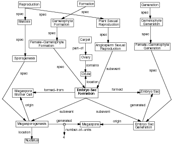
(c)
| ARGENTINA
|
| (a) Example entry from the World Fact-book (excerpt). |
|
(b) Country description, from http://www.elca.org/dgm/country_packet/packets/latin_america-caribbean/argentina/desc.html |
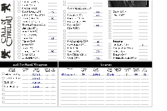 |
| (a) Character Page |
| Mitzo Rotis is a prodigious professor. Born in Boston,
MA, as young as 25 year-old, he is already an acclaimed
anthropologist, well know by his persuasive speeches and
psychological set ups. A weak, average sized person, a fire
accident early on his life marked his physical appearance and
his psyche (he is afraid of fire in all its forms). This is not a
problem for the psychoanalytic Dr. Rotis, that is still able to
charm any audience with his never ending conversation and
most varied knowledge, ranging from Physics to Greek. |
| (b) Character Description |
Acker, L. and Porter, B. W. (1994). Extracting viewpoints from knowledge bases. In Proceedings of the National Conference on Artificial Intelligence, pages 547–552.
André, E. and Rist, T. (1995). Generating coherent presentations employing textual and visual material. AI Review, 9:147–165.
Androutsopoulos, I., Kokkinaki, V., Dimitromanolaki, A., Calder, J., Oberlander, J., and Not, E. (2001). Generating multilingual personalized descriptions of museum exhibits: the M-PIRO project. In Proceedings of the International Conference on Computer Applications and Quantitative Methods in Archaeology, Gotland, Sweden.
Ansari, D. and Hirst, G. (1998). Generating warning instructions by planning accidents and injuries. In Proceedings of the Ninth International Workshop on Natural Language Generation (INLG-98), pages 118–127, Niagara-on-the-Lake, Ontario.
Bangalore, S. and Rambow, O. (2000). Exploiting a probabilistic hierarchical model for generation. In COLING, 2000, Saarbrücken, Germany.
Barzilay, R., Elhadad, N., and McKeown, K. (2002). Inferring strategies for sentence ordering in multidocument news summarization. Journal of Artificial Intelligence Research, 17:35–55.
Barzilay, R., Elhadad, N., and McKeown, K. R. (2001). Sentence ordering in multidocument summarization. In Proceedings of the Conference on Human Language Technologies HLT, San Diego (CA), USA.
Barzilay, R. and Lee, L. (2002). Bootstrapping lexical choice via multiple-sequence alignment. In Proceedings of the 2002 Conference on Empirical Methods for Natural Language Processing EMNLP-2002, Philadelphia, PA.
Barzilay, R. and Lee, L. (2004). Catching the drift: Probabilistic content models, with applications to generation and summarization. In Susan Dumais, D. M. and Roukos, S., editors, HLT-NAACL 2004: Main Proceedings, pages 113–120, Boston, Massachusetts, USA. Association for Computational Linguistics.
Barzilay, R., Reiter, E., and Siskind, J. M., editors (2003). Workshop on Learning Word Meaning from Non-Linguistic Data, Edmonton, Canada. ACL.
Basu, S., Mooney, R. J., Pasupuleti, K. V., and Ghosh, J. (2001). Using lexical knowlege to evaluate the novelty of rules mined from text. In Proceedings of NAACL Workshop on WordNet and Other Lexical Resources, pages 144–149, Pittsburgh, PA.
Bateman, J. A. and Teich, E. (1995). Selective information presentation in an integrated publication system: an application of genre-driven text generation. Information Processing and Management, 5(31):753–768.
Belz, A. (2000). Computational Learning of Finite-State Models for Natural Language Processing. PhD thesis, University of Sussex.
Berners-Lee, T., Hendler, J., and Lassila, O. (2001). The semantic web. Scientific American.
Bikel, D. M., Schwartz, R., and Weischedel, R. M. (1999). An algorithm that learns what’s in a name. Machine Learning, 34(1-3):211–231.
Bontcheva, K. and Wilks, Y. (2001). Dealing with dependencies between content planning and surface realisation in a pipeline generation architecture. In Proceedings International Joint Conference on Artificial Intelligence (IJCAI-2001).
Bontcheva, K. and Wilks, Y. (2004). Automatic report generation from ontologies: the miakt approach. In Nineth International Conference on Applications of Natural Language to Information Systems (NLDB’2004), Manchester, UK.
Bouayad-Agha, N., Power, R., and Scott, D. (2000). Can text structure be incompatible with rhetorical structure? In Proceedings of First International Conference on Natural Language Generation (INLG-2000), Mitzpe Ramon, Israel.
Buchanan, B. and Wilkins, D. (1993). Readings in Knowledge Acquisition and Learning. Morgan Kaufmann.
Cahill, L., Doran, C., Evans, R., Mellish, C., Paiva, D., Reape, M., Scott, D., and Tipper, N. (2000). Reinterpretation of an existing NLG system in a generic generation architecture. In Proceedings of First International Conference on Natural Language Generation (INLG-2000), Mitzpe Ramon, Israel.
Cheng, H. and Mellish, C. (2000). Capturing the interaction between aggregation and text planning in two generation systems. In Proceedings of the First International Conference on Natural Language Generation (INLG-2000), Mitzpe Ramon, Israel.
Cheng, H., Poesio, M., Henschel, R., and Mellish, C. (2001). Corpus-based NP modifier generation. In Proceedings of the Second Meeting of the North American Chapter of the Association for Computational Linguistics (NAACL-2001), Carnegie Mellon University, Pittsburgh, PA.
Chieu, H. L., Ng, H. T., and Lee, Y. K. (2003). Closing the gap: Learning-based information extraction rivaling knowledge-engineering methods. In Hinrichs, E. and Roth, D., editors, Proceedings of the 41st Annual Meeting of the Association for Computational Linguistics, pages 216–223, Sapporo, Japan.
Cohen, W. (1996). Learning trees and rules with set-valued features. In Proceedings of the 14th joint American Association for Artificial Intelligence and IAAI Conference (AAAI/IAAI-96), pages 709–716. American Association for Artificial Intelligence.
Cohen, W., Schapire, R., and Singer, Y. (1999). Learning to order things. Journal of Artificial Intelligence, 10:243–270.
Columbia, N. G. (2001). Columbia statistical generation day. http://www.cs.columbia.edu/nlp/sgd/.
Corston-Oliver, S., Gamon, M., Ringger, E., and Moore, R. (2002). An overview of Amalgam: A machine-learned generation module. In Proceedings of the Second International Conference on Natural Language Generation (INLG-2002), pages 33–40, Ramapo Mountains, NY.
Cox, R., O’Donnell, M., and Oberlander, J. (1999). Dynamic versus static hypermedia in museum education: an evaluation of ILEX, the intelligent labelling explorer. In Proceedings of the Artificial Intelligence in Education conference (AI-ED99), Le Mans.
Dalal, M., Feiner, S., McKeown, K. R., Pan, S., Zhou, M., Hollerer, T., Shaw, J., Feng, Y., and Fromer, J. (1996). Negotiation for automated generation of temporal multimedia presentations. In Proceedings of ACM Multimedia ’96, Philadelphia (PA), USA.
Dale, R., Milosavljevic, M., and Oberlander, J. (1997). The web as dialogue: the role of natural language generation in hypertext. In Proceedings of the AAAI Symposium on Natural Language Processing and the World Wide Web, Stanford University.
Dale, R., Oberlander, J., Milosavljevic, M., and Knott, A. (1998). Integrating natural language generation with hypertext to produce dynamic documents. Interacting with Computers, 11:109–135.
Dalianis, H. (1999). Aggregation in natural language generation. Journal of Computational Intelligence, 15(4):384–414.
Danlos, L., Gaiffe, B., and Roussarie, L. (2001). Document structuring á la SDRT. In Proceedings of the Eighth European Workshop on Natural Language Generation (EWNLG 2001/ACL 2001), pages 11–20, Toulouse, France.
Daumé III, H. and Marcu, D. (2004). A phrase-based HMM approach to document/abstract alignment. In Proceedings of EMNLP, Barcelona, Spain.
Dempster, A. P., Laird, N. M., and Rubin, D. B. (1977). Maximum likelihood from incomplete data via the EM algorithm. Journal of Royal Statistical Society, Series B (Methodological), 39(1).
Dimitromanolaki, A. and Androutsopoulos, I. (2003). Learning to order facts for discourse planning in natural language generation. In Proceedings of the Ninth European Workshop on Natural Language Generation, Tenth Conference of the European Chapter of the Association for Computational Linguistics (EACL 2003), Budapest, Hungary.
Duboue, P. A. (2004). Indirect supervised learning of content selection logic. In Proceedings of the Third International Conference in Natural Language Generation (INLG-2004), pages 41–50, New Forest, UK. ACL SIGGEN.
Duboue, P. A. (2005). Openschema: A declarative implementation of document structuring schemata. Technical report, Columbia University, Computer Science Department.
Duboue, P. A. and McKeown, K. R. (2002). Content planner construction via evolutionary algorithms and a corpus-based fitness function. In Proceedings of the Second International Conference on Natural Language Generation (INLG-2002), Ramapo Mountains, NY.
Duboue, P. A. and McKeown, K. R. (2003a). Statistical acquisition of content selection rules for natural la nguage generation. In Proceedings of the 2003 Conference on Empirical Methods for Natural Language Processing EMNLP-2003, Sapporo, Japan.
Duboue, P. A. and McKeown, K. R. (2003b). Statistical acquisition of content selection rules for natural language generation. Technical report, Columbia University, Computer Science Department.
Duboue, P. A., McKeown, K. R., and Hatzivassiloglou, V. (2003). ProGenIE: Biographical descriptions for intelligence analysis. In Proceedings of the NSF/NIJ Symposium on Intelligence and Security Informatics, volume 2665 of Lecture Notes in Computer Science, pages 343–345, Tucson, Arizona. Springer-Verlag.
Dunning, T. (1993). Accurate methods for the statistics of surprise and coincidence. Computational Linguistics, 19(1).
Dupont, P. (1994). Regular grammatical inference from positive and negative samples by genetic search: The gig method. In Proceedings of ICGI-94: Grammatical Inference and Applications, Second International Colloquium. Springer, Berlin.
Durbin, R., Eddy, S., Krogh, A., and Mitchison, G. (1998). Biological sequence analysis. Cambridge Univeristy Press.
Elhadad, M. and Robin, J. (1996). An overview of SURGE: A reusable comprehensive syntactic realization component. Technical report, Dept of Mathematics and Computer Science, Ben Gurion University, Beer Sheva, Israel.
Fellegi, I. P. and Sunter, A. B. (1969). A theory for record linkage. Journal of the American Statistical Association, 64:1183–1210.
Filatova, E. and Hatzivassiloglou, V. (2003). Domain-independent detection, extraction, and labeling of atomic events. In Proceedings of RANLP, Borovetz, Bulgaria.
Filatova, E. and Hatzivassiloglou, V. (2004). A formal model for information selection in multi-sentence text extraction. In Proceedings of COLING, Geneva, Switzerland.
Fisher, D., Soderland, S., McCarthy, J., Feng, F., and Lehnert, W. (1995). Description of the UMass system as used for MUC-6. In Kaufman, M., editor, Proceedings of the Sixth Message Understanding Conference (MUC-6), pages 127–140, San Francisco.
Gusfield, D. (1997). Algorithms on strings, trees and sequences: computer science and computational biology. Cambridge University Press, Cambridge.
Hertz, J., Krogh, A., and Palmer, R. (1991). Introduction to the Theory of Neural Computation. Addision Wesley.
Hovy, E. and Maier, E. (1995). Parsimonious or profligate: How many and which discourse structure relations? Master’s thesis, ISI-USC. Unpublished ms.
Hovy, E. H. (1988). Planning coherent multisentential text. In Proceedings of the 26th Annual Meeting of the Association for Computational Linguistics (ACL-88), Buffalo, N.Y. Association for Computational Linguistics.
Hovy, E. H. (1993). Automated discourse generation using discourse structure relations. Artificial Intelligence. (Special Issue on Natural Language Processing).
Huang, X. (1994). Planning argumentative texts. In Proceedings of 15th International Conference on Computational Linguistics (COLING-94), Kyoto, Japan.
Hudak, J. and McClure, M. (1999). A comparative analysis of computational motif–detection methods. In Altman, R., Dunker, A. K., Hunter, L., Klein, T. E., and Lauderdale, K., editors, Proceedings of the Pacific Symposium on Biocomputing (PSB-99), pages 138–149, New Jersey. World Scientific.
Jaffar, J. and Lassez, J.-L. (1986). Constraint logic programming. Technical report, University of Melbourne. Also in the proceedings of POPL’87 (1987).
Jansche, M. (2003). Parametric models of linguistic count data. In Hinrichs, E. and Roth, D., editors, Proceedings of the 41st Annual Meeting of the Association for Computational Linguistics, pages 288–295.
Jing, H. and McKeown, K. R. (1999). The decomposition of human-written summary sentences. In Proceedings of SIGIR’99, University of Berkeley (CA), USA.
Jing, H. and McKeown, K. R. (2000). Cut and paste based text summarization. In Proceedings of the 1st Conference of the North American Chapter of the Association for Computational Linguistics (NAACL’00), Seattle, Washington.
John, G. H. and Langley, P. (1995). Estimating continuous distributions in bayesian classifiers. In Proceedings of the Eleventh Conference on Uncertainty in Artificial Intelligence, pages 338–345. Morgan Kaufmann, San Mateo.
Jurafsky, D. and Martin, J. H. (2000). Speech and Language Processing, An Introduction to Natural Language Processing, Computational Linguistics, and Speech Recognition. Prentice-Hall.
Kamps, T., Kleinz, J., Bateman, J., and Reichenberger, K. (2001). Towards constructive text, diagram, and layout generation for information presentation. Computational Linguistics, 27(3):409–449.
Kan, M.-Y. and McKeown, K. R. (2002). Corpus-trained text generation for summarization. In Proceedings of the Second International Conference on Natural Language Generation (INLG-2002), Ramapo Mountains, NY.
Karamanis, N. (2003). Entity Coherence for Descriptive Text Structuring. PhD thesis, School of Informatics, University of Edinburgh.
Karamanis, N. and Manurung, H. M. (2002). Stochastic text structuring using the principle of continuity. In Proceedings of the Second International Conference on Natural Language Generation (INLG-2002), Ramapo Mountains, NY.
Kibble, R. and Power, R. (1999). Using centering theory to plan coherent texts. In Proceedings of the 12th Amsterdam Colloquium.
Kim, S., Alani, H., Hall, W., Lewis, P., Millard, D., Shadbolt, N., and Weal, M. (2002). Artequakt: Generating tailored biographies with automatically annotated fragments from the web. In Proceedings of the Semantic Authoring, Annotation and Knowledge Markup Workshop in the 15th European Conference on Artificial Intelligence, Lyon, France.
Kittredge, R., Korelsky, T., and Rambow, O. (1991). On the need for domain communication language. Computational Intelligence, 7(4):305–314.
Knight, K. and Hatzivassiloglou, V. (1995). Two-level, many-paths generation. In Proceedings of the Conference of the Association for Computational Linguistics (ACL-95).
Knott, A. and Dale, R. (1993). Using linguistic phenomena to motivate a set of rhetorical relations. Technical Report RP-39, HCRC.
Knott, A., O’Donnell, M., Oberlander, J., and Mellish, C. (1997). Defeasible rules in content selection and text structuring. In Proceedings of the Sixth European Workshop on Natural Language Generation, pages 50–60, Duisburg, Germany.
Koza, J. (1994). Genetic Programming II. MIT Press.
Kukich, K. (1983). Knowledge Based Report Generation: A Knowledge-Engineering Approach to Natural Language Report Generation. PhD thesis, University of Pittsburgh.
Kupiec, J. M., Pedersen, J., and Chen, F. (1995). A trainable document summarizer. In Fox, E. A., Ingwersen, P., and Fidel, R., editors, Proceedings of the 18th Annual International ACM SIGIR Conference on Research and Development in Information Retrieval (SIGIR-95), pages 68–73, Seattle, Washington.
Langkilde, I. (2000). Forest-based statistical sentence generation. In Proceedings of the First Meeting of the North American Chapter of the Association for Computational Linguistics (NAACL-2000), Seattle, WA.
Langkilde, I. and Knight, K. (1998). The practical value of n-grams in generation. In Proceedings of the Ninth International Natural Language Generation Workshop (INLG-98), Niagara-on-the-lake, Ontario.
Lapata, M. (2003). Probabilistic text structuring: Experiments with sentence ordering. In Proceedings of the 41st Meeting of the Association of Computational Linguistics, pages 545–552, Sapporo, Japan.
Lassila, O. and Swick, R. R. (1999). Resource Description Framework (RDF) model and syntax specification. http://www.w3.org/TR/REC-rdf-syntax. W3C Recommendation.
Lavoie, B. and Rambow, O. (1997). A fast and portable realizer for text generation systems. In Proceedigns of the Conference on Applied Natural Language Processing (ANLP-97), Washington, DC.
le Cessie, S. and van Houwelingen, J. (1992). Ridge estimators in logistic regression. Applied Statistics, 41(1):191–201.
Lebanon, G. and Lafferty, J. (2002). Combining rankings using conditional probability models on permutations. In Sammut, C. and A. Hoffmann, e., editors, Proceedings of the 19th International Conference on Machine Learning, San Francisco, CA. Morgan Kaufmann Publishers.
Lester, J. and Porter, B. (1997). Developing and empirically evaluating robust explanation generators: The KNIGHT experiments. Computational Linguistics, 23(1):65–101.
Levin, E. and Pieraccini, R. (1997). A stochastic model of computer-human interaction for learning dialogue strategies. In Proceedings of Eurospeech, pages 1883–1886, Rhodes, Greece.
Lim, J.-G. (1992). Planning in AI and text planning in natural language generation. Technical report, Columbia University, Computer Science Department.
Malouf, R. (2000). The order of prenominal adjectives in natural language generation. In Proceedings of the 38th Annual Meeting of the Association for Computational Linguistics (ACL-2000), Hong Kong.
Mann, W. C. and Thompson, S. A. (1988). Rhetorical structure theory: Toward a functional theory of text organization. Text, 8(3):243–281.
Marcu, D. (1997). From local to global coherence: A bottom-up approach to text planning. In Proceedings of Fourteenth National Conference on Artificial Intelligence (AAAI-97), pages 450–456.
Marcu, D. (2000). The Theory and Practice of Discourse Parsing and Summarization. The MIT Press. ISBN 0-262-13372-5.
Marcu, D., Carlson, L., and Watanabe, M. (2000). An empirical study in multilingual natural language generation: what should a text planner do? In Proceedings of the First International Conference on Natural Language Generation (INLG-2000), Mitzpe Ramon, Israel.
Marcu, D. and Echihabi, A. (2002). An unsupervised approach to recognizing discourse relations. In Proceedings of the 40th Annual Meeting of the Association for Computational Linguistics (ACL-2002), Philadelphia, PA.
Maybury, M. (1988). Genny: A knowledge based text generation system. In Proceedings of the RIAO Conference on User-Oriented Content-Based Text and Image Handling, pages 849–862, MIT, Cambridge, MA.
McKeown, K. R. (1983). Text Generation: Using Discourse Strategies and Focus Constraints to Generate Natural Language Text. PhD thesis, University of Pennsylvania, Computer Science Department.
McKeown, K. R. (1985). Text Generation: Using Discourse Strategies and Focus Constraints to Generate Natural Language Text. Cambridge University Press, Cambridge, England.
McKeown, K. R., Jordan, D., Feiner, S., Shaw, J., Chen, E., Ahmad, S., Kushniruk, A., and Patel, V. (2000). A study of communication in the cardiac surgery intensive care unit and its implications for automated briefing. In Proceedings of the Annual Meeting of the American Medical Informatics Association (AMIA-2000).
McKeown, K. R. and Pan, S. (1999). Prosody modeling in concept-to-speech generation: Methodological issues. Philosophical Transactions of the Royal Society.
Mellish, C., Knott, A., Oberlander, J., and O’Donnell, M. (1998). Experiments using stochastic search for text planning. In Proceedings of the Ninth International Workshop on Natural Language Generation (INLG-98), pages 98–107, Niagra-on-the-Lake, Ontario, Canada.
Michalewicz, Z. (1992). Genetic Algorithms + Data Structures = Evolution Programs. Springer-Verlag, New York.
Milosavljevic, M. (1999). Maximising the Coherence of Descriptions via Comparison. PhD thesis, Macquarie University, Sydney, Australia.
Minton, S., editor (1993). Machine learning methods for planning. Morgan Kaufmann series in machine learning. M. Kaufmann, San Mateo, CA.
Mitchell, T. M. (1997). Machine Learning. McGraw-Hill.
Moore, J. and Paris, C. L. (1988). Constructing coherent text using rhetorical relations. In Proceedings of the Tenth Annual Conference of the Cognitive Science Society, pages 637–643, Montreal, Quebec.
Moore, J. D. and Paris, C. L. (1993). Planning text for advisory dialogues: Capturing intentional and rhetorical information. Computational Linguistics, 19(4):651–695.
Moore, J. D. and Pollack, M. E. (1992). A problem for RST: The need for multi-level discourse analysis. Computational Linguistics, 18(4):537–544.
Moore, J. M. and Swartout, W. (1991). Natural Language Generation in Artificial Intelligence and Computational Linguistics, chapter A Reactive Approach to Explanation: Taking the User’s Feedback into Account. Kluwer Academic Publisher.
Müller, A. and Kutschekmanesch, S. (1995). Using abductive inference and dynamic indexing to retrieve multimedia SGML documents. In Ruthven, I., editor, Final Workshop on Multimedia Information Retrieval (Miro ’95), Glasgow, Scotland.
Muslea, I. (1997). A general-purpose AI planning system based on the genetic programming paradigm. In Late Breaking Papers at GP-97, pages 157–164.
Nenkova, A. and Passonneau, R. (2004). Evaluating content selection in summarization: the Pyramid method. In Susan Dumais, D. M. and Roukos, S., editors, HLT-NAACL 2004: Main Proceedings, Boston, Massachusetts, USA.
Neumann, G. (1997). Applying explanation-based learning to control and speeding–up natural language generation. In Proceedings of the 35th Conference of the Association for Computational Linguistics (ACL-97), Madrid, Spain.
O’Donnell, M., Mellish, C., Oberlander, J., and Knott, A. (2001). ILEX: an architecture for a dynamic hypertext generation system. Natural Language Engineering, 7:225–250.
Oh, A. and Rudnicky, A. (2000). Stochastic language generation for spoken dialogue systems. In Proceedings of the ANLP/NAACL 2000 Workshop on Conversational Systems, pages 27–32, Seattle, WA.
Pan, S. and McKeown, K. R. (1999). Word informativeness and automatic pitch accent modeling. In Proceedings of the 1999 Conference on Empirical Methods in Natural Language Processing and Very Large Corpora (EMNLP/VLC-99), University of Maryland, College Park (MD), USA.
Pan, S. and Shaw, J. (2004). Segue: A hybrid case-based surface natural language generator. In Proceedings of the Third International Conference in Natural Language Generation (INLG-2004), pages 130–140, New Forest, UK. ACL SIGGEN.
Pang, B., Lee, L., and Vaithyanathan, S. (2002). Thumbs up? sentiment classification using machine learning techniques. In Proceedings of the 2002 Conference on Empirical Methods in Natural Language Processing (EMNLP-2002), pages 79–86.
Paris, C. L. (1987). The Use of Explicit User Models in Text Generation: Tailoring to a User’s Level of Expertise. PhD thesis, Columbia University.
Platt, J. (1998). Advances in Kernel Methods - Support Vector Learning, chapter Fast Training of Support Vector Machines using Sequential Minimal Optimization. MIT Press.
Poesio, M., Henschel, R., and Kibble, R. (1999). Statistical NP generation: A first report. In Proceedings of the ESSLLI Workshop on NP Generation, Utrecht.
Porayska-Pomsta, K., Mellish, C., and Pain, H. (2000). Aspects of speech act categorisation: Towards generating teachers language. International Journal of Artificial Intelligence in Education, 11:254–272.
Power, R. (2000). Planning texts by constraint satisfaction. In Proceedings of the 18th International Conference on Computational Linguistics (COLING-2000), pages 642–648, Saarbruecken, Germany.
Quinlan, J. R. (1993). C4.5: Programs for Machine Learning. Morgan Kaufmann, San Mateo, California.
Radev, D., Teufel, S., Saggion, H., Lam, W., Blitzer, J., Çelebi, A., Qi, H., Drabek, E., and Liu, D. (2002). Evaluation of text summarization in a cross-lingual information retrieval framework. Technical report, Center for Language and Speech Processing, Johns Hopkins University, Baltimore, MD. Johns Hopkins University 2001 summer workshop final report.
Radev, D. R. and McKeown, K. R. (1997). Building a generation knowledge source using internet-accessible newswire. In Proceedings of the Fifth Conference on Applied Natural Language Processing (ANLP-97), pages 221–228, Washington (DC), USA.
Rahm, E. and Do, H. H. (2000). Data cleaning: Problems and current approaches. IEEE Bulletin of the Technical Committee on Data Engineering, 23(4).
Rambow, O. (1999). Extended discourse plan operators. In Proceedings of LORID-99, International Workshop on Text Representation, University of Edinburgh.
Ratnaparkhi, A. (2000). Trainable methods for surface natural language generation. In Proceedings of the First Meeting of the North American Chapter of the Association of Computational Linguistics (NAACL-2000), pages 194–201, Seattle, WA.
Reiter, E. (2000). Pipelines and size constraints. Computational Linguistics, 26:251–259.
Reiter, E., Cawsey, A., Osman, L., and Roff, Y. (1997). Knowledge acquistion for content selection. In Proceedings of the Sixth European Workshop on Natural Language Generation (INLG-97), pages 117–126, Duisberg, Germany.
Reiter, E. and Dale, R. (2000). Building Natural Language Generation Systems. Cambridge University Press.
Reiter, E., Robertson, R., and Osman, L. (2000). Knowledge acquisition for natural language generation. In Proceedings of the Fist International Conference on Natural Language Generation (INLG-2000), pages 217–224.
Reiter, E. and Sripada, S. (2002). Should corpora texts be gold standards for NLG? In Proceedings of Second International Conference on Natural Language Generation INLG-2002, pages 97–104, Arden House, NY.
Ries, K. (1999). HMM and neural network based speech act detection. In International Conference on Acoustics and Signal Processing (ICASSP-99), Phoenix, Arizona, USA.
Rigoutsos, I. and Floratos, A. (1998). Combinatorial pattern discovery in biological sequences: the teiresias algorithm. Bioinformatics, 14(1):55–67.
Riloff, E. (1993). Automatically constructing a dictionary for information extraction. In Press, A. P. . M., editor, Proceedings of the 11th National Conference on Artificial Intelligence, pages 811–816.
Robin, J. and McKeown, K. R. (1993). Corpus analysis for revision-based generation of complex sentences. In Proceedings of the 11th National Conference on Artificial Intelligence (AAAI-93), pages 365–372, Washington, DC.
Rösner, D. and Stede, M. (1992). Techdoc: A system for the automatic production of multilingual technical documents. In Proceedings of KONVENS ’92. Springer-Verlag.
Schiffman, B. (2002). Building a resource for evaluating the importance of sentences. In Proceedings of the Third International Conference on Language Resources and Evaluation.
Schiffman, B., Mani, I., and Concepcion, K. J. (2001). Producing biographical summaries: Combining linguistic knowledge with corpus statistics. In Proceedings of the 39th Annual Meeting of the Association for Computational Linguistics (ACL-EACL 2001), Toulouse, France.
Shaw, J. (1998). Clause aggregation using linguistic knowledge. In Proceedings of Ninth International Workshop on Natural Language Generation (INLG-98), pages 138–147.
Shaw, J. (2001). Clause Aggregation: An approach to generating concise text. PhD thesis, Columbia University.
Shaw, J. and Hatzivassiloglou, V. (1999). Ordering among premodifiers. In Proceedings of the 37th Annual Meeting of the Association for Computational Linguistics (ACL-99), pages 135–143, University of Maryland, College Park (MD), USA.
Siddharthan, A. (2003). Syntactic Simplification and Text Cohesion. PhD thesis, University of Cambridge.
Singh, S., Litman, D. J., Kearns, M., and Walker, M. (2002). Optimizing dialogue management with reinforcement learning: Experiments with the NJFun system. Journal of Artificial Intelligence Research, 16:105–133.
Smadja, F. and McKeown, K. R. (1990). Automatically extracting and representing collocations for language generation. In Proceedings of the Annual Meeting of the Association for Computational Linguistics (ACL-90).
Sripada, S. and Reiter, E. (2003). Learning the meaning and usage of time phrases from a parallel text-data corpus. In Proceedings of the HLT-NAACL03 Workshop on Learning Word Meaning from Non-Linguistic Data, pages 78–85.
Sripada, S., Reiter, E., Hunter, J., and Yu, J. (2003). Exploiting a parallel text-data corpus. In Proceedings of Corpus Linguistics 2003.
Sripada, S. G., Reiter, E., Hunter, J., and Yu, J. (2001). A two-stage model for content determination. In ACL/EWNLG-2001, pages 3–10, Toulouse, France.
Stent, A. (2000). Rhetorical struture in dialog. In Proceedings of the Second International Natural Language Generation Conference (INLG-2000). student paper.
Taskar, B., Segal, E., and Koller, D. (2001). Probabilistic clustering in relational data. In Proceedings of the 17th International Joint Conference on Artificial Intelligence, pages 870–876, Seattle, Washington.
Teich, E. and Bateman, J. A. (1994). Towards an application of text generation in an integrated publication system. In Proceedings of the Seventh International Workshop on Natural Language Generation, Kennebunkport, Maine, USA, June 21-24, 1994, pages 153–162, Kennebunkport, Maine, USA.
Turney, P. (2002). Thumbs up or thumbs down? semantic orientation applied to unsupervised classification of reviews. In Proceeding of the 2002 Conference of the Association for Computational Linguistics (ACL-2002).
Van Halteren, H. and Teufel, S. (2003). Examining the consensus between human summaries: initial experiments with factoid analysis. In HLT/NAACL-2003 Workshop on Automatic Summarization, Edmonton, Canada.
van Rijsbergen, C. J. (1979). Information Retrieval. Butterworths, London, 2nd edition.
Vander Linden, K. (1992). The expression of local rhetorical relations in instructional text. In Proceedings of the 30th Annual Meeting of the Association for Computational Linguistics (ACL-92), pages 318–320, Newark, Delaware.
Vander Linden, K. (1995). On graphical procedural representations. Technical report, ITRI, University of Brighton.
Varges, S. (2003). Instance-based Natural Language Generation. PhD thesis, Institute for Communicating and Collaborative Systems, School of Informatics, University of Edinburgh.
Varges, S. and Mellish, C. (2001). Instance-based natural language generation. In Proceedings of the Second Meeting of the North American Chapter of the Association for Computational Linguistics (NAACL-2001), Carnegie Mellon University, Pittsburgh, PA.
Walker, M. A. and Rambow, O. (1994). The role of cognitive modeling in achieving communicative intentions. In Proceedings of the Seventh International Workshop on Natural Language Generation (INLG-94), Kennebunkport, ME.
Walker, M. A., Rambow, O., and Rogati, M. (2002). Training a sentence planning for spoken dialogue using boosting. Computer Speech and Language.
Washio, T. and Motoda, H. (2003). State of the art of graph-based data mining. SIGKDD Explor. Newsl., 5(1):59–68.
Witten, I. H. and Frank, E. (2000). Data Mining: Practical Machine Learning Tools and Techniques with Java Implementations. Morgan Kaufmann Publishers.
Wolz, U. (1990). An object-oriented approach to content planning for text generation. Technical Report Technical Report: CUCS-004-90, Columbia University, Department of Computer Science, New York, NY 10027.
Young, M. R. (1996). A developer’s guide to the longbow discourse planning system. Technical report, Intelligent Systems Program, University of Pittsburgh. version 1.0, alpha 12.
Young, M. R. and Moore, J. D. (1994). DPOCL: A principled approach to discourse planning. In Proceedings of the Seventh International Workshop on Text Generation (INLG-94), Kennebunkport, ME.
Young, S. J. (2002). Talking to machines (statistically speaking). In Proceedings of the International Conference on Spoken Language Processing (ICSLP-2002), Denver, Colorado.
Yu, H. and Hatzivassiloglou, V. (2003). Towards answering opinion questions: Separating facts from opinions and identifying the polarity of opinion sentences. In Proceedings of the 2003 Conference on Empirical Methods for Natural Language Processing EMNLP-2003, Sapporo, Japan.
Zhou, H. and Grefenstette, J. J. (1986). Induction of finite automata by genetic algorithms. In Proceedings of the 1986 International Conference on Systems, Man and Cybernetics, pages 170–174.
Zhou, L., Burgoon, J. K., and Twitchell, D. P. (2003). A longitudinal analysis of language behavior of deception in e-mail. In Chen, H., Miranda, R., Zeng, D. D., Demchak, C. C., Schroeder, J., and Madhusudan, T., editors, Proceedings of Intelligence and Security Informatics, First NSF/NIJ Symposium (ISI-2003), volume 2665 of Lecture Notes in Computer Science, pages 102–110, Tucson, AZ, USA. Springer.
Zock, M. (1986). LE FIL D’ARIANE: ou les Grammaires de Texte comme guide dans l’organisation et l’expression de la pensée en langue maternelle et/ou etrangère. Technical report, UNESCO, Paris. 110 pages.
Zukerman, I., Korb, K., and McConarchy, R. (1996). Perambulations on the way to an architecture for a nice argument generator. In Notes of the ECAI-96 Workshop on Gaps and Bridges: “New Directions in Planning and Natural Language Generation”, pages 31–36, Budapest, Hungary.
Following (Mitchell, 1997), pages 146-147, to compute whether the differences observed
between two machine learning methods are statistically significant, it is necessary to compute
their mean and an estimator for their standard deviation. I will use a three-fold cross-validation
to compute these differences. Therefore, given three folds (Tr1,Te1), (Tr2,Te2), (Tr3,Te3) and
two system variants A, B, each variant is trained in (Tr1 +Te1), (Tr2 +Te2), (Tr3 +Te3)
and tested in Te1,Te2,Te3:
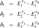
Then we compute the average, defined as

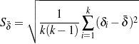
The true difference in the two variants lies in the interval

where is the mean of the differences and S is an estimator for the standard deviation defined above and t2,N depends on the confidence interval (N%), and it is given by the following table:
| N= | 90% | 95% | 98% | 99% |
| t= | 2.92 | 4.30 | 6.96 | 9.92 |
In the following tables, I will consider the difference between two variants to be statistically significant if the interval over described above does not includes the zero. Please note these differences are over error rates and in this thesis I have focused in differences on F-measure. I am using these differences to shed light about whether the different variants are performing in a way that can be due purely to chance or not.
| Variant | Partition 1 | Partition 2 | Partition 3 | ||||||||||||||||||
| size=439 | size=410 | size=280 | |||||||||||||||||||
0 |
error=0.17 |
error=0.14 |
error=0.21 |
||||||||||||||||||
1 |
error=0.18 |
error=0.17 |
error=0.23 |
||||||||||||||||||
2 |
error=0.17 |
error=0.14 |
error=0.20 |
||||||||||||||||||
3 |
error=0.16 |
error=0.15 |
error=0.2 |
||||||||||||||||||
4 |
error=0.17 |
error=0.14 |
error=0.19 |
||||||||||||||||||
biography.com corpus. Table A.1.
Baseline stat. signif. different from Variant 4, conf.: 74.658
Baseline stat. signif. different from Variant 3, conf.: 66.476
Baseline stat. signif. different from Variant 2, conf.: 76.322
Variant 2 stat. signif. different from Variant 4, conf.: 68.240
Variant 1 stat. signif. different from Baseline, conf.: 96.969
Variant 1 stat. signif. different from Variant 4, conf.: 93.142
Variant 1 stat. signif. different from Variant 3, conf.: 96.605
Variant 1 stat. signif. different from Variant 2, conf.: 92.958
variant4-variant3, no conclusion could be arrived.
variant3-variant2, no conclusion could be arrived.
| Variant | Partition 1 | Partition 2 | Partition 3 | ||||||||||||||||||
| size=509 | size=1031 | size=515 | |||||||||||||||||||
0 |
error=0.07 |
error=0.10 |
error=0.06 |
||||||||||||||||||
2 |
error=0.07 |
error=0.09 |
error=0.07 |
||||||||||||||||||
3 |
error=0.07 |
error=0.09 |
error=0.06 |
||||||||||||||||||
4 |
error=0.06 |
error=0.09 |
error=0.06 |
||||||||||||||||||
s9.com corpus. Table A.2.
Baseline stat. signif. different from Variant 3, conf.: 61.629
Variant 2 stat. signif. different from Variant 4, conf.: 77.157
Variant 2 stat. signif. different from Variant 3, conf.: 67.628
baseline-variant4, no conclusion could be arrived.
baseline-variant2, no conclusion could be arrived.
variant4-variant3, no conclusion could be arrived.
| Variant | Partition 1 | Partition 2 | Partition 3 | ||||||||||||||||||
| size=685 | size=519 | size=378 | |||||||||||||||||||
0 |
error=0.16 |
error=0.16 |
error=0.18 |
||||||||||||||||||
2 |
error=0.16 |
error=0.16 |
error=0.18 |
||||||||||||||||||
3 |
error=0.16 |
error=0.15 |
error=0.19 |
||||||||||||||||||
4 |
error=0.16 |
error=0.14 |
error=0.18 |
||||||||||||||||||
imdb.com corpus. Table A.3.
Baseline stat. signif. different from Variant 4, conf.: 63.724
Baseline stat. signif. different from Variant 2, conf.: 81.351
Variant 3 stat. signif. different from Variant 4, conf.: 87.437
baseline-variant3, no conclusion could be arrived.
variant4-variant2, no conclusion could be arrived.
variant3-variant2, no conclusion could be arrived.
| Variant | Partition 1 | Partition 2 | Partition 3 | ||||||||||||||||||
| size=2110 | size=2048 | size=916 | |||||||||||||||||||
0 |
error=0.08 |
error=0.08 |
error=0.13 |
||||||||||||||||||
2 |
error=0.08 |
error=0.09 |
error=0.14 |
||||||||||||||||||
3 |
error=0.08 |
error=0.08 |
error=0.13 |
||||||||||||||||||
4 |
error=0.08 |
error=0.08 |
error=0.13 |
||||||||||||||||||
wikipedia.org corpus. Table A.4.
Variant 3 stat. signif. different from Baseline, conf.: 57.515
Variant 2 stat. signif. different from Baseline, conf.: 92.959
Variant 2 stat. signif. different from Variant 4, conf.: 85.757
Variant 2 stat. signif. different from Variant 3, conf.: 91.401
baseline-variant4, no conclusion could be arrived.
variant4-variant3, no conclusion could be arrived.
| Variant | Partition 1 | Partition 2 | Partition 3 | ||||||||||||||||||
| size=439 | size=410 | size=280 | |||||||||||||||||||
0 |
error=0.23 |
error=0.24 |
error=0.22 |
||||||||||||||||||
4 |
error=0.24 |
error=0.29 |
error=0.25 |
||||||||||||||||||
4 |
error=0.29 |
error=0.31 |
error=0.34 |
||||||||||||||||||
biography.com corpus. Table A.5.
Variant 4 stat. signif. different from Baseline, conf.: 96.421
Variant 4 stat. signif. different from Select-All/Select-None, conf.: 89.501
Select-All/Select-None stat. signif. different from Baseline, conf.: 89.539
| Variant | Partition 1 | Partition 2 | Partition 3 | ||||||||||||||||||
| size=509 | size=1031 | size=515 | |||||||||||||||||||
0 |
error=0.09 |
error=0.13 |
error=0.09 |
||||||||||||||||||
4 |
error=0.08 |
error=0.07 |
error=0.07 |
||||||||||||||||||
4 |
error=0.10 |
error=0.14 |
error=0.09 |
||||||||||||||||||
s9.com corpus. Table A.6.
Baseline stat. signif. different from Select-All/Select-None, conf.: 77.382
Variant 4 stat. signif. different from Baseline, conf.: 95.858
Variant 4 stat. signif. different from Select-All/Select-None, conf.: 80.741
| Variant | Partition 1 | Partition 2 | Partition 3 | ||||||||||||||||||
| size=685 | size=519 | size=378 | |||||||||||||||||||
0 |
error=0.20 |
error=0.15 |
error=0.23 |
||||||||||||||||||
4 |
error=0.23 |
error=0.17 |
error=0.23 |
||||||||||||||||||
4 |
error=0.24 |
error=0.29 |
error=0.24 |
||||||||||||||||||
imdb.com corpus. Table A.7.
Variant 4 stat. signif. different from Baseline, conf.: 75.658
Variant 4 stat. signif. different from Select-All/Select-None, conf.: 64.636
Select-All/Select-None stat. signif. different from Baseline, conf.: 82.845
| Variant | Partition 1 | Partition 2 | Partition 3 | ||||||||||||||||||
| size=2110 | size=2048 | size=916 | |||||||||||||||||||
0 |
error=0.08 |
error=0.08 |
error=0.16 |
||||||||||||||||||
4 |
error=0.09 |
error=0.09 |
error=0.18 |
||||||||||||||||||
4 |
error=0.12 |
error=0.11 |
error=0.20 |
||||||||||||||||||
wikipedia.org corpus. Table A.8.
Variant 4 stat. signif. different from Baseline, conf.: 96.205
Variant 4 stat. signif. different from Select-All/Select-None, conf.: 95.816
Select-All/Select-None stat. signif. different from Baseline, conf.: 88.590